Determining stability by cobwebbing linear approximations around equilibria
Determining stability by cobwebbing linear approximations around equilibria.
One way to explore the stability of an equilibrium of a discrete dynamical system is to use cobwebbing to see whether or not solutions converge to the equilibrium. If you can always find a solution that moves away from the equilibrium, even for initial conditions really close to the equilibrium, then the equilibrium is unstable. If, on the other hand, all solutions that start close enough to the equilibrium stay close, or even approach, the equilibrium, then the equilibrium is stable.
We'll use this technique to find conditions on discrete dynamical systems for equilibria to be stable. First, we'll look at linear dynamical systems. Then, we'll see if we can generalize our condition to nonlinear dynamical systems.
Linear dynamical systems
No constant term
The simplest form of a linear discrete dynamical system is one where there is no constant term, i.e., a dynamical system of the form \begin{align} z_{n+1} = a z_n, \quad \text{for $n=0,1,2,\ldots$} \label{linearnoconstant}\tag{1} \end{align} where $a$ is a parameter. This form of dynamical system includes exponential growth and decay, which occurs when $a$ is positive. But, here we will also allow $a$ to be negative, so we'll get a larger range of behavior.
Our goal is to determine the equilibria of model \eqref{linearnoconstant} and their stability as a function of the parameter $a$. We can do this graphically, using the cobwebbing applet. You'll need to do some translations in the notation because the applet is set up for a model of the form $x_{n+1}=f(x_n)$. Just use $z$ rather than $x$ and notice that for model \eqref{linearnoconstant}, we are using the function $f(z)=az$.
To find the equilibria using the cobwebbing applet:
- Enter the right hand side of model \eqref{linearnoconstant} in the “$f(x)=$” box in the applet. Type $x$ for $z_n$. You'll have to choose a particular numerical value for $a$ and type that number rather than “$a$”.
- Find the equilibria as the intersections between the graph of $z_{n+1}=f(z_n)$ (in blue) and the graph of the diagonal $z_{n+1}=z_n$ (in red).
- To determine the stability, you need to find out what happens to the trajectory (the solution) of initial conditions $z_0$ near the equilibria. (In the applet, the initial condition is denoted by $x_0$.) If the initial condition $z_0$ is close to the equilibrium, and the distance from the equilibrium to the iterates $z_n$ doesn't get larger, then the equilibrium is stable. If, on the other hand, the distance from the equilibrium to the iterates $z_n$ gets larger, even if you make $z_0$ really close to the equilibrium, then the equilibrium is unstable. (Of course, if you make $z_0$ exactly equal to the equilibrium, the iterates $z_n$ will always stay at the equilibrium, by definition of an equilibrium. So, making $z_0$ equal to the equilibrium doesn't tell us about stability.)
Follow this procedure for different values of $a$, both positive and negative, to determine for which values of $a$ the equilibria are stable, and for which values of $a$ the equilibria are unstable. In the end, we want a set of conditions so that, given any value of $a$, you can determine the equilibria of model \eqref{linearnoconstant} and their stability.
Adding a constant term
The next step is to determine what happens to the equilibria when one adds a constant term to the dynamical system, yielding a dynamical system of the form \begin{align} y_{n+1} = b y_n + c, \quad \text{for $n=0,1,2,\ldots$} \label{linearwithconstant}\tag{2} \end{align} where $b$ and $c$ are parameters, which can be positive or negative.
Repeat the same procedure for this model. In this case, find the equilibria algebraically, by making both $y_n$ and $y_{n+1}$ be the same quantity and solving for that quantity. You might find that, when the constant term $c$ is not zero, there is a particular value of $b$ where there are no equilibria.
For the cases where there are equilibria, we want to determine how their stability depends on the parameters $b$ and $c$. You can use the above steps to determine the stability, remembering that one has to use $x$ rather than $y$ in the applet.
In the end, what we want is conditions on $b$ and $c$ for the stability and instability of the equilibria. Also state the condition on $b$ and $c$ for the special case where there are no equilibria. How do the results compare to what you found for the case without a constant term? In particular, what is the influence of the constant term on the stability of the equilibria?
Nonlinear dynamical systems
Linear dynamical systems are the simplest type to understand. For a discrete dynamical system of the form \begin{align} x_{n+1} = f(x_n) \quad \text{for $n=0,1,2,\ldots$} \label{generalsystem}\tag{3} \end{align} the situation gets much more complicated when $f(x)$ is a nonlinear function. Such nonlinear discrete dynamical systems can exhibit very complicated behavior (even chaos).
Finding a linear approximation around equilibria
Since this behavior is too complicated for us to deal with right now, we are going to see if we can understand some aspects of a nonlinear system by pretending it is a linear system. We'll use this trick to understand the condition for the stability of equilibria.
Graphically, finding equilibria of nonlinear systems isn't any more difficult than for linear systems. We just graph $x_{n+1}=f(x_n)$ (in blue, below) on the same axes as the diagonal $x_{n+1}=x_n$ (in red, below). Equilibria are the points where the blue curve intersects the red line.
The stability of an equilibrium is defined based on what happens to solutions near the equilibrium; to determine stability, we just need to know whether or not solutions near the equilibrium move away from it. We'll exploit this fact by simplifying the form of $f(x)$ for values of $x$ around an equilibrium. We'll make a linear approximation of $f$ around an equilibrium so that we can apply our previous results. At this point, we won't ask you to find the linear approximation. Instead, we made an applet to do the work for you.
The following applet is a modification of the cobweb applet that can also compute a linear approximation to $f(x)$ around an equilibrium. To calculate a linear approximation, click the “find E” and click near an equilibrium, i.e., near where the graph of $f$ (in blue) intersects the diagonal (in red). If all goes well, the applet will find the equilibrium $E$ and display its value underneath the button.
When the applet finds an equilibrium, it also calculates a tangent line to the function around that equilibrium and displays it as a green line. The tangent line is a linear function that matches the function very closely around the equilibrium. The tangent line is the linear approximation we will need. The slope of this tangent line is displayed below the value of the equilibrium.
To see how well the linear approximation matches the function around the equilibrium, click the “center E” button, which will center the equilibrium in the middle of the window. Then, click the zoom in button “+” many times to zoom in on the equilibrium. What do you notice about the relationship between the graph of $f$ (in blue) and the graph of the tangent line (in green) as you zoom in on the equilibrium? The property you are observing is what it means for a line to be tangent to the graph of $f$.
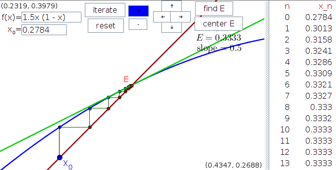
Cobwebbing and linear approximations around equilibria. Cobwebbing provides a way to visualize how a linear approximation to a function captures the behavior of its iteration near equilibria. Clicking the “iterate” button shows the behavior of the function iteration $x_n = f(x_{n-1})$ in a cobweb plot. The iterates $x_n$ are also displayed in the list at the right. To find an equilibrium (defined by $E=f(E)$), click the “find E” button, then click near a point where the graph of $f(x)$ (blue curve) intersects the diagonal $y=x$ (red line). If an equilibrium is found, the value of $E$ is displayed and a red point appears at the coordinates $(E,E)$. The linear approximation of $f$ around $E$ appears as a green line that is tangent to the graph of $f$ at the red point, and the value of its slope is displayed. If you click “center E,” the red point representing $E$ will be centered, and you can zoom in with the + button to see the behavior of $f$ right around $E$. What do you notice about the relationship of the linear approximation in green and the function in blue when you zoom in on the equilibrium? What does this say about the ability of the linear approximation to predict the behavior of $f$ around $E$? You can change the function $f(x)$ by typing a new function in the box. You can change the initial point $x_0$ by typing a new value in the box or dragging the blue point. You can zoom in and out with the + and - buttons as well as pan in different directions with the buttons labeled by arrows.
Using the linear approximation to determine stability
Now, you have all the pieces to determine the stability of the equilibrium of a nonlinear discrete dynamical system. You simply need to put together three pieces of information. The first is your result for the stability of an equilibrium of a linear dynamical system. The second is the fact that stability of an equilibria is defined in terms of points that are very close to the equilibrium. The third piece of information is the fact that the linear approximation calculated by the applet is a good approximation to the function $f$ for points close to the equilibrium.
To come up with the criteria and test if it really works, you'll need to test many different functions $f(x)$. Feel free to come up with your own functions to test. If you like, here are some examples to try: $f(x)=1.5x(1-x)$, $f(x) = x+0.3x(x-1)(x-3)$, $f(x) = x-0.05(x-1))(x-3)(x-5)$, $f(x)= (x-1)^2$. It's also a good idea to try a whole family of functions that vary by changing a parameter. That way you can quantitatively test your criteria. For example, the function $f(x)=1.5x(1-x)$ is one member of the family of functions $f(x)=rx(1-x)$ for parameter $r$. Try this function not only for $r=1.5$, but for other values of $r$, like $r=2$, $r=2.8$, or $r=3.2$ (and values in between). If you are really brave, try this function with $r=4$. With these tests, you should be able to convince yourself whether or not you've come up with the right criteria for the stability of a nonlinear discrete dynamical system.
Thread navigation
Math 1241, Fall 2020
- Previous: Problem set: The tangent line as a linear approximation
- Next: Problem set: Determining stability by cobwebbing linear approximations around equilibria
Math 201, Spring 22
Similar pages
- The idea of stability of equilibria for discrete dynamical systems
- A model of chemical pollution in a lake
- Equilibria in discrete dynamical systems
- A graphical approach to finding equilibria of discrete dynamical systems
- The idea of a dynamical system
- An introduction to discrete dynamical systems
- Developing an initial model to describe bacteria growth
- Bacteria growth model exercises
- Bacteria growth model exercise answers
- Exponential growth and decay modeled by discrete dynamical systems
- More similar pages