The idea of a probability distribution
Overview
A random variable is a variable that is subject to variations due to random chance. One can think of a random variable as the result of a random experiment, such as rolling a die, flipping a coin, picking a number from a given interval. The idea is that, each time you perform the experiment, you obtain a sample of the random variable. Since the variable is random, you expect to get different values as you obtain multiple samples. (Some values might be more likely than others, as in an experiment of rolloing two six-sided die and recording the sum of the resulting two numbers, where obtaining a value of 7 is much more likely than obtaining value of 12.) A probability distribution is a function that describes how likely you will obtain the different possible values of the random variable.
It turns out that probability distributions have quite different forms depending on whether the random variable takes on discrete values (such as numbers from the set $\{1,2,3,4,5,6\}$) or takes on any value from a continuum (such as any real number in the interval $[0,1]$). Despite their different forms, one can do the same manipulations and calculations with either discrete or continuous random variables. The main difference is usually just whether one uses a sum or an integral.
Discrete probability distribution
A discrete random variable is a random variable that can take on any value from a discrete set of values. The set of possible values could be finite, such as in the case of rolling a six-sided die, where the values lie in the set $\{1,2,3,4,5,6\}$. However, the set of possible values could also be countably infinite, such as the set of integers $\{0, 1, -1, 2, -2, 3, -3, \ldots \}$. The requirement for a discrete random variable is that we can enumerate all the values in the set of its possible values, as we will need to sum over all these possibilities.
For a discrete random variable $X$, we form its probability distribution function by assigning a probability that $X$ is equal to each of its possible values. For example, for a six-sided die, we would assign a probability of $1/6$ to each of the six options. In the context of discrete random variables, we can refer to the probability distribution function as a probability mass function. The probability mass function $P(x)$ for a random variable $X$ is defined so that for any number $x$, the value of $P(x)$ is the probability that the random variable $X$ equals the given number $x$, i.e., \begin{align*} P(x) = \Pr(X = x). \end{align*} Often, we denote the random variable of the probability mass function with a subscript, so may write \begin{align*} P_X(x) = \Pr(X = x). \end{align*}
For a function $P(x)$ to be valid probability mass function, $P(x)$ must be non-negative for each possible value $x$. Moreover, the random variable must take on some value in the set of possible values with probability one, so we require that $P(x)$ must sum to one. In equations, the requirenments are \begin{gather*} P(x) \ge 0 \quad \text{for all $x$}\\ \sum_x P(x) = 1, \end{gather*} where the sum is implicitly over all possible values of $X$.
For the example of rolling a six-sided die, the probability mass function is \begin{gather*} P(x) = \begin{cases} \frac{1}{6} & \text{if $x \in \{1,2,3,4,5,6\}$}\\ 0 & \text{otherwise.} \end{cases} \end{gather*}
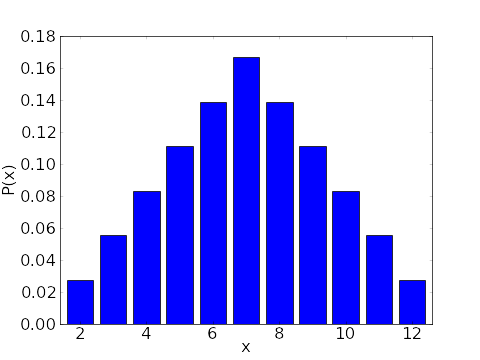
If we rolled two six-sided dice, and let $X$ be the sum, then $X$ could take on any value in the set $\{2,3,4,5,6,7,8,9,10,11,12\}$. The probability mass function for this $X$ is \begin{gather*} P(x) = \begin{cases} \frac{1}{36} & \text{if $x \in \{2,12\}$}\\ \frac{2}{36}=\frac{1}{18} & \text{if $x \in \{3,11\}$}\\ \frac{3}{36}=\frac{1}{12} & \text{if $x \in \{4,10\}$}\\ \frac{4}{36}=\frac{1}{9} & \text{if $x \in \{5,9\}$}\\ \frac{5}{36} & \text{if $x \in \{6,8\}$}\\ \frac{6}{36} =\frac{1}{6} & \text{if $x = 7$}\\ 0 & \text{otherwise.} \end{cases} \end{gather*} $P(x)$ is plotted as a bar graph in the following figure.
Continuous probability distribution
A continuous random variable is a random variable that can take on any value from a continuum, such as the set of all real numbers or an interval. We cannot form a sum over such a set of numbers. (There are too many, since such a continuum is uncountable.) Instead, we replace the sum used for discrete random variables with an integral over the set of possible values.
For a continuous random variable $X$, we cannot form its probability distribution function by assigning a probability that $X$ is exactly equal to each value. The probability distribution function we must use in the case is called a probability density function, which essentially assigns the probability that $X$ is near each value. For intuition behind why we must use such a density rather than assigning individual probabilities, see the page that describes the idea behind the probability density function.
Given the probability density function $\rho(x)$ for $X$, we determine the probability that $X$ is in any set $A$ (i.e., that $X \in A$ (confused?)) by integrating $\rho(x)$ over the set $A$, i.e., \begin{gather*} \Pr(X \in A) = \int_A \rho(x)dx. \end{gather*} Often, we denote the random variable of the probability density function with a subscript, so may write \begin{gather*} \Pr(X \in A) = \int_A \rho_X(x)dx. \end{gather*}
The definition of this probability using an integral gives one important consequence for continuous random variables. If the set $A$ contains just a single element, we can immediately see that the probability that $X$ is equal to that one value is exactly zero, as the integral over a single point is zero. For a continuous random variable $X$, the probability that $X$ is any single value is always zero.
In other respects, the probability density function of a continuous random variables behaves just like the probability mass function for a discrete random variable, where we just need to use integrals rather than sums. For a function $\rho(x)$ to be valid probability density function, $\rho(x)$ must be non-negative for each possible value $x$. Just as for discrete random variable, a continuous random variable must take on some value in the set of possible values with probability one. In this case, we require that $\rho(x)$ must integral to one. In equations, the requirenments are \begin{gather*} \rho(x) \ge 0 \quad \text{for all $x$}\\ \int \rho(x)dx = 1, \end{gather*} where the integral is implicitly over all possible values of $X$.
For examples of continuous random variables and their associated probability density functions, see the page on the idea behind the probability density function.