Plotting line graphs in R
The basic plot command
Imagine that in R, we created a variable $t$ for time points and a variable $z$ that showed a quantity that is decaying in time.
> t=0:10
> z= exp(-t/2)
The simplest R command to plot $z$ versus $t$ is
> plot(t,z)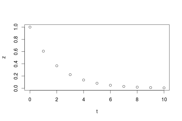
Without any other arguments, R plots the data with circles and uses the variable names for the axis labels. The plot command accepts many arguments to change the look of the graph. Here, we use type="l" to plot a line rather than symbols, change the color to green, make the line width be 5, specify different labels for the $x$ and $y$ axis, and add a title (with the main argument).
> plot(t,z, type="l", col="green", lwd=5, xlab="time", ylab="concentration", main="Exponential decay")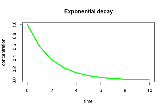
A line plot with multiple series
Imagine that you wanted to plot not only $z$ but also a variable $w$ that was increasing with time.
> w = 0.1*exp(t/3)One way to plot separate lines for both $z$ and $w$ is to first plot $z$ with the plot and then add a line for $w$ with the lines command.
> plot(t,z, type="l", col="green", lwd=5, xlab="time", ylab="concentration")
> lines(t, w, col="red", lwd=2)
> title("Exponential growth and decay")
> legend(2,1,c("decay","growth"), lwd=c(5,2), col=c("green","red"), y.intersp=1.5)
The last two lines add a title (since it wasn't added with a main argument of the plot command) and a legend. The first two arguments to the legend command are its position, the next is the legend text, and the following two are just vectors of the same arguments of the plot and lines commands, as R requires you to specify them again for the legend. (The last y.intersp argument just increases the vertical spacing of the legend.)
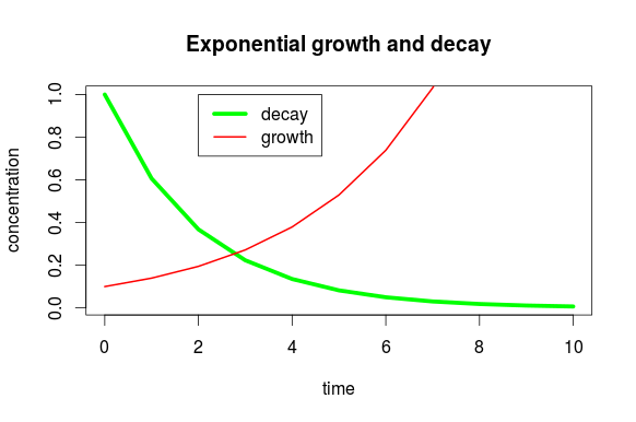
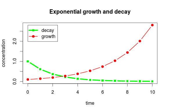
Notice that the range of the plot does not expand to include all of the line plotted by the lines command. By default, the plot sets the axis limits to fit the data given it. If you can manual specify the axis limits with the xlim or ylim arguments. Adding the argument ylim = range(w,z) will ensure that the $y$-axis limits include all the data from both $z$ and $w$. The following commands will show all the data of $w$. These commands also show how to add both points as well as lines by specifying type="b". The symbols used for the points are specified by the pch (plotting character) argument.
> plot(t,z, type="b", col="green", lwd=5, pch=15, xlab="time", ylab="concentration", ylim=range(w,z))
> lines(t, w, type="b", col="red", lwd=2, pch=19)
> title("Exponential growth and decay")
> legend(0,2.8,c("decay","growth"), lwd=c(5,2), col=c("green","red"), pch=c(15,19), y.intersp=1.5)