The idea of a probability density function
An initial thought experiment
I'm thinking of a number, let's call it $X$, between 0 and 10 (inclusive). If I don't tell you anything else, what would you imagine is the probability that $X=0$? That $X=4$? Assuming that I don't have any preference for any particular number, you'd imagine that the probability of each of the eleven integers $0,1,2,\ldots, 10$ is the same. Since all the probabilities must add up to 1, a logical conclusion is to assign a probability of $1/11$ to each of the 11 options, i.e., you'd assume that the probability that $X=i$ is $1/11$ for any integer $i$ from 0 to 10, which we write as \begin{gather*} \Pr(X=i) = \frac{1}{11} \qquad \text{for } i=0,1,2, \ldots, 10. \end{gather*} Implicit in this description is the assumption that the probability that $X$ is any other number $x$ is zero. (Here we make a distinction between the random number $X$ and the variable $x$ which can stand for any fixed number.) We can write this implicit assumption as \begin{gather*} \Pr(X=x) = 0 \qquad \text{if $x$ is not one of } \{0,1,2, \ldots, 10\}. \end{gather*}
What would change if instead I told you that I was thinking of a number $X$ between 0 and 1 (inclusive)? You might assume that I was thinking of either the number 0 or the number 1, and you'd assign a probability 1/2 to both options. Or, you might guess that I had more than two options in mind. There was nothing in what I said that forces you to conclude that I was thinking of an integer. Maybe I was thinking of 1/2, or 1/4, or 7/8. Once you start going down that road, the possibilities are endless. I could be thinking of any fraction between 0 and 1. But who said I was limiting myself to rational numbers? I could even be thinking of irrational numbers like $1/\sqrt{2}$ or $\pi/5$. If we allow the possibility that the number $X$ could any real number in the interval $[0,1]$, then there are clearly an infinite number of possibilities. (Of course, I could have been thinking of non-integers for the number betwen 0 and 10 as well, but most people would think I was referring to integers in that case.)
Since we don't want to assume that I am favoring any particular number, then we should insist that the probability is the same for each number. In other words, the probability that the random number $X$ is any particular number $x \in [0,1]$ (confused?) should be some constant value; let's use $c$ to denote this probability of any single number. But, now we run into trouble due to the fact that there are an infinite number of possibilities. If each possibility has the same probability $c$ and the probabilities must add up to 1 and there are an infinite number of possibilities, what could the individual probability $c$ possibly be? If $c$ were any finite number greater than zero, once we add up an infinite number of the $c$'s, we must get to infinity, which is definitely larger than the required sum of 1. In order to prevent the sum from blowing up to infinity, we must have $c$ be infinitesimally small, i.e., we must insist that $c=0$. The probability that I chose any particular number, such as the probability that $X$ equals $1/2$, must be equal to zero. We can write this as \begin{gather*} \Pr(X=x) = 0 \qquad \text{for any real number $x$}. \end{gather*}
What went wrong here? We know all probabilities must not be zero, because we know that the total probability must add up to one. In fact, were know that, somehow, there must be something special for the probability of numbers $0 \le x \le 1$. We know that $X$ is somewhere in that interval with probability one, and the probability that $X$ is outside that interval is zero.
The probability density
It turns out, for the case where we allow $X$ to be any real number, we are just approaching the question in the wrong way. We should not ask for the probability that $X$ is exactly a single number (since that probability is zero). Instead, we need to think about the probability that $x$ is close to a single number.
We capture the notion of being close to a number with a probability density function which is often denoted by $\rho(x)$. If the probability density around a point $x$ is large, that means the random variable $X$ is likely to be close to $x$. If, on the other hand, $\rho(x)=0$ in some interval, then $X$ won't be in that interval.
To translate the probability density $\rho(x)$ into a probability, imagine that $I_x$ is some small interval around the point $x$. Then, assuming $\rho$ is continuous, the probability that $X$ is in that interval will depend both on the density $\rho(x)$ and the length of the interval: \begin{gather} \Pr(X \in I_x) \approx \rho(x) \times \text{Length of $I_x$}. \label{eq:densityapprox} \end{gather} We don't have a true equality here, because the density $\rho$ may vary over the interval $I_x$. But, the approximation becomes better and better as the interval $I_x$ shrinks around the point $x$, as $\rho$ will be come closer and closer to a constant inside that small interval. The probability $\Pr(X \in I_x)$ approaches zero as $I_x$ shrinks down to the point $x$ (consistent with our above result for single numbers), but the information about $X$ is contained in the rate that this probability goes to zero as $I_x$ shrinks.
In general, to determine the probability that $X$ is in any subset $A$ of the real numbers, we simply add up the values of $\rho(x)$ in the subset. By “add up,” we mean integrate the function $\rho(x)$ over the set $A$. The probability that $X$ is in $A$ is precisely \begin{gather} \Pr(x \in A) = \int_A \rho(x)dx. \label{eq:density} \end{gather}
For example, if $I$ is the interval $I=[a,b]$ with $a \le b$, then the probability that $a \le X \le b$ is \begin{gather*} \Pr(x \in I) = \int_I \rho(x)dx = \int_a^b \rho(x)dx. \end{gather*}
For a function $\rho(x)$ to be a probability density function, it must satisfy two conditions. It must be non-negative, so the that integral \eqref{eq:density} is always non-negative, and it must integrate to one, so that the probability of $X$ being something is one: \begin{gather*} \rho(x) \ge 0 \quad \text{for all $x$}\\ \int \rho(x) dx = 1, \end{gather*} where the integral is implicitly taken over the whole real line.
Equation \eqref{eq:density} is the right way to define a probability density function. However, if we aren't worrying about being too precise or about discontinuities in $\rho$, we may sometimes state that \begin{gather*} \Pr(X \in (x,x+dx)) = \rho(x)dx. \end{gather*} Here, we are thinking of $dx$ as being an infinitesimally small number so that $(x,x+dx)$ is an infinitesimally small interval $I_x$ around $x$, in which case the approximation \eqref{eq:densityapprox} becomes exact, at least if $\rho$ is continuous.
Examples
Example 1
Returning to the opening example of a number in the interval $[0,1]$, we can let $X$ be given by a uniform distribution in the interval $[0,1]$. The resulting probability density function of $X$ is given by \begin{gather*} \rho(x) = \begin{cases} 1 & \text{if $x \in [0,1]$}\\ 0 & \text{otherwise} \end{cases} \end{gather*} and is illustrated in the following figure.
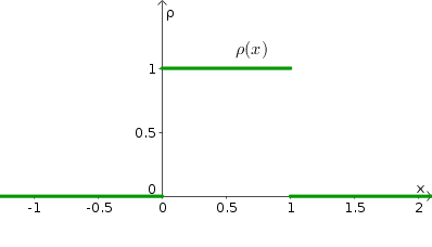
The function $\rho(x)$ is a valid probability density function since it is non-negative and integrates to one.
If $I$ is an interval contained in $[0,1]$, say $I=[a,b]$ with $0 \le a \le b \le 1$, then $\rho(x)=1$ in the interval and \begin{align*} \Pr(x \in I) &= \int_I \rho(x)dx\\ &=\int_I 1 \, dx\\ &= \int_a^b 1\,dx = b-a=\text{Length of $I$}. \end{align*} For any interval $I$, $\Pr(x \in I)$ is equal to the length of the intersection of $I$ with the interval $[0,1]$.
Example 2
If \begin{gather*} \rho(x) = \begin{cases} x & \text{if $0 \lt x \lt 1$}\\ 2-x & \text{if $1 \lt x \lt 2$}\\ 0 & \text{otherwise}, \end{cases} \end{gather*} then $\rho(x)$ is a triangular probability density function centered around 1.
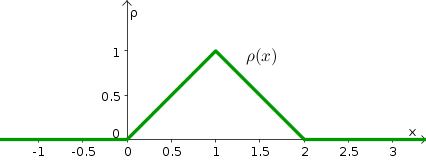
You can verify that $\int \rho(x)dx=1$ so $\rho$ is a valid density. The density is largest near 1. If a random variable $X$ is given by this density, you can verify that \begin{align*} \Pr\left(\frac{1}{2} \lt X \lt \frac{3}{2}\right) = \int_{1/2}^{3/2} \rho(x)dx = \frac{3}{4}. \end{align*}
In this definition of $\rho(x)$ it doesn't matter that we defined $\rho(1)=0$. The density at a single point doesn't matter. We would get the same random variable if we used the density \begin{gather*} \rho(x) = \begin{cases} x & \text{if $0 \lt x \le 1$}\\ 2-x & \text{if $1 \lt x \lt 2$}\\ 0 & \text{otherwise} \end{cases} \end{gather*} so that $\rho(1)=1$. This second definition is a little nicer because $\rho$ is continuous. However, the value of an integral doesn't depend on the value of its integrand at just one point, so given the definition of equation \eqref{eq:density}, the probability of the random variable $X$ being in any set is unchanged if we change $\rho$ at just one point (or at any finite number of points).
Example 3
One very important probability density function is that of a Gaussian random variable, also called a normal random variable. The probability density function looks like a bell-shaped curve.
One example is the density \begin{gather*} \rho(x) = \frac{1}{\sqrt{2\pi}} e^{-x^2/2}, \end{gather*} which is graphed below. One has to do some tricks to verify that indeed $\int \rho(x)dx=1$.
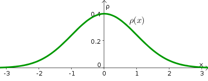
It turns out that Gaussian random variables show up naturally in many contexts in probability and statistics.