The degree distribution of a network
A network can be an exceedingly complex structure, as the connections among the nodes can exhibit complicated patterns. One challenge in studying complex networks is to develop simplified measures that capture some elements of the structure in an understandable way.
One such simplification is to ignore any patterns among different nodes, but just look at each node separately. If one zooms in onto a node and ignores all other nodes, the only thing one can see is how many connections the node has, i.e., the degree of the node.
Undirected networks
If we restrict ourselves to undirected networks for the moment, then the degree of a node $i$ is just the number of connections it has. In terms of the adjacency matrix $A$, the degree of node $i$ is just the some of the $i$th row of $A$, \begin{gather*} k_i=\sum_j a_{ij}, \end{gather*} where the sum is over all nodes in the network.
We can then obtain some insight into the network structure by throwing out information about the network except for the degrees of its nodes. By counting how many nodes have each degree, we form the degree distribution $P_{\text{deg}}(k)$, defined by \begin{gather*} P_{\text{deg}}(k) = \text{fraction of nodes in the graph with degree $k$}. \end{gather*}
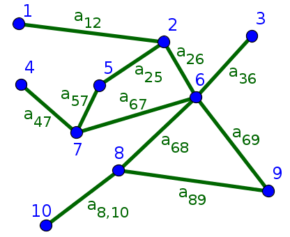
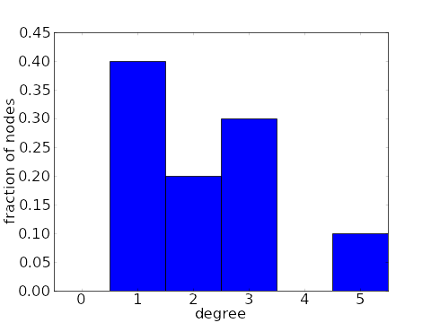
For this undirected network, the degrees are $k_1=1$, $k_2=3$, $k_3=1$, $k_4=1$, $k_5=2$, $k_6=5$, $k_7=3$, $k_8=3$, $k_9=2$, and $k_{10}=1$. Its degree distribution is $P_{\text{deg}}(1)=2/5$, $P_{\text{deg}}(2)=1/5$, $P_{\text{deg}}(3)=3/10$, $P_{\text{deg}}(5)=1/10$, and all other $P_{\text{deg}}(k)=0$.
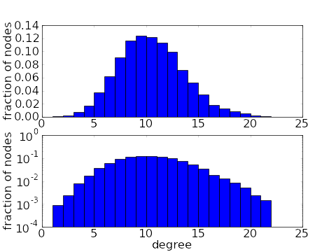
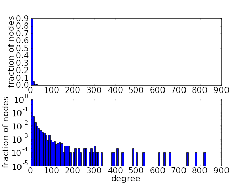
The degree distribution clearly captures only a small amount of information about a network. But that information still gives important clues into structure of a network. For example, in the simplest types of networks, one would find that most nodes in the network had similar degrees (see first pair of plots, below). However, real world networks usually have very different degree distributions. In a real world network, most nodes have a relatively small degree, but a few nodes will have very large degree, being connected to many other nodes. These large-degree nodes are often referred to as hubs, in analogy to transportation network such as one connecting airports, where some very large hub airport have connections to many others. For example, in the second pair of plots, below, the average degree is around 7, but 3/4 of the nodes have a degree of 3 or less. The average is brought up to 7 by the presence of a few hubs with degrees in the high hundreds. Such a degree distribution is said to have a long tail.
As demonstrated above, a measure as simple as the degree distribution can give us a glimpse into the structure of a network and distinguish different types of networks. Obviously, the degree distribution captures only a small amount of the network structure, as it ignores how the nodes are connected to each other.
For a particular network, one might wonder how much of the structure is captured by the degree distribution. One way to investigate this question is to construct another network using just the information contained in the degree distribution and compare this new network with the original. One can use the configuration model to create a network from a degree distribution and examine this question.
The configuration model assumes that nodes connect to other nodes without regard to the relationship between their degrees. However, one could imagine a network where the hubs preferentially tended to connect to other hubs. Or, the opposite might be true, and hubs could preferentially connect to nodes of low degree. Hence, to capture more information than just the degree distribution, one might look at degree correlations.
Directed networks
The degree distribution of directed networks is a bit more complicated it was for undirected networks. The reason is that the degree of a node in a directed network cannot be captured by a single number. If we zoom in on a node in a directed network, we will see some edges coming into the node and some edges going out from the node. One could just ignore the direction of the edges and just add up the total number of edges (obtaining the total degree, below), but that throws out a lot of information. An incoming edge and an outgoing edge can mean very different things, and one might want to keep that distinction.
Instead, one can just add up the incoming connections and outgoing connections separately, obtaining two numbers for the degree of a node. The in-degree of node $i$ is the total number of connections onto node $i$, and is the sum of the $i$th row of the adjacency matrix \begin{gather*} k_i^{\text{in}}=\sum_j a_{ij}. \end{gather*} On the other hand, the out-degree of node $i$ is the total number of connections coming from node $i$ and is the sum of the $i$th column of the adjacency matrix \begin{gather*} k_i^{\text{out}}=\sum_j a_{ji}. \end{gather*} In both cases, the sum is over all nodes $j$ of the network. We can add the in- and out-degrees to get the total number of connections of a node, or its total degree \begin{gather*} k_i^{\text{tot}} = k_i^{\text{in}} + k_i^{\text{out}}. \end{gather*}
With two degrees, the degree distribution becomes a two-dimensional distribution, so that $P_{\text{deg}}(k^{\text{in}},k^{\text{out}} ) = $ the fraction of nodes in the graph with in-degree $k^{\text{in}}$ and out-degree $k^{\text{out}}$. We can't plot this two-dimensional degree-distribution as a simple bar plot. We can use a surface plot or a color plot to visualize this information.
If we want to use bar plots, we could look at the marginal degree distributions. One of the marginal degree distributions is the in-degree distribution, $P_{\text{deg}}^{\text{in}}(k^{\text{in}}) = $ the fraction of nodes in the graph with in-degree $k^{\text{in}}$. The other is the out-degree distribution, $P_{\text{deg}}^{\text{out}}(k^{\text{out}}) = $ the fraction of nodes in the graph with out-degree $k^{\text{out}}$. A third one-dimensional distribution that could be useful is the total degree distribution, $P_{\text{deg}}^{\text{tot}}(k^{\text{tot}}) = $ the fraction of nodes in the graph with total degree $k^{\text{tot}}$.
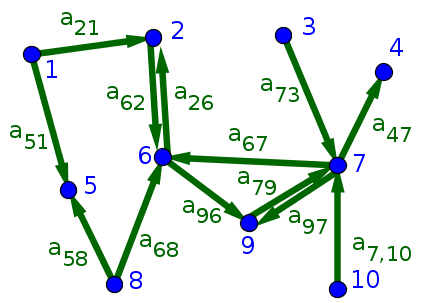
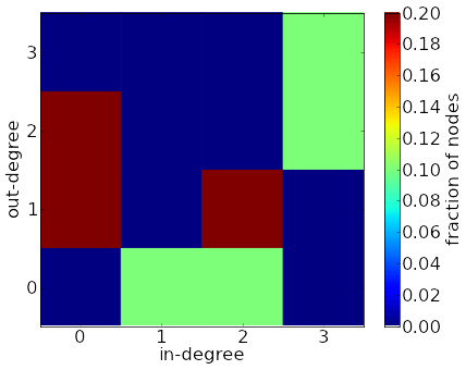
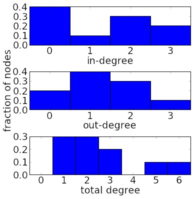
For the above network, the in- and out-degrees are $(k_1^{\text{in}},k_1^{\text{out}})=(0,2)$, $(k_2^{\text{in}},k_2^{\text{out}})=(2,1)$, $(k_3^{\text{in}},k_3^{\text{out}})=(0,1)$, $(k_4^{\text{in}},k_4^{\text{out}})=(1,0)$, $(k_5^{\text{in}},k_5^{\text{out}})=(2,0)$, $(k_6^{\text{in}},k_6^{\text{out}})=(3,2)$, $(k_7^{\text{in}},k_7^{\text{out}})=(3,3)$, $(k_8^{\text{in}},k_8^{\text{out}})=(0,2)$, $(k_9^{\text{in}},k_9^{\text{out}})=(2,1)$, and $(k_{10}^{\text{in}},k_{10}^{\text{out}})=(0,1)$. A two-dimensional histogram of these values is plotted with the color plot. The marginal degree distributions, involving just the in-degrees or just the out-degrees, are shown in the first two bar plots. The third bar plot shows the total degree distribution, based on the total degrees $k_1^{\text{tot}}=2$, $k_2^{\text{tot}}=3$, $k_3^{\text{tot}}=1$, $k_4^{\text{tot}}=1$, $k_5^{\text{tot}}=2$, $k_6^{\text{tot}}=5$, $k_7^{\text{tot}}=6$, $k_8^{\text{tot}}=2$, $k_9^{\text{tot}}=3$, and $k_{10}^{\text{tot}}=1$.
The marginal degree distributions involving just the in-degree or just the out-degree are a lot simpler to deal with. So, rather than dealing with the full two-dimensional degree distribution, one could just study the marginal distributions separately. An implicit assumption in this approach is that one is not concerned about correlations between a node's in-degree and a node's out-degree. Essentially, one assumes that if one node has a large in-degree (is an incoming hub) and another nodes has a small in-degree, both nodes are equally likely to have a large out-degree (be a outgoing hub).
The assumption of uncorrelated in- and out-degrees might make sense for some networks, but it certainly doesn't have to be true. One can easily imagine a network where the incoming hubs are also the outgoing hubs, or the reverse case where the incoming hubs are completely distinct from the outgoing hubs.
The correlation between in- and out-degree can make a large difference to the effective properties of the network. Imagine a network where the nodes are people and the directed edges indicate which people talk to which other people. The incoming hubs then correspond to people (the listeners) who are listening to lots of others . The outgoing hubs correspond to people (the talkers) who are talking to lots of others. If one wants a message to spread quickly across the network, then one would want talkers to be the listeners. On the other hand, as can occur from time to time, when the listeners aren't talking and the talkers aren't listening, information is not efficently passed along the network.
The strong influence of the correlation between in- and out-degree can be seen by the fact that it determines the largest eigenvalue of the adjacency matrix.1 This eigenvalue, in turn, influences the properties of dynamical systems that evolve on the network, such as the synchronization of networked oscillators.2,3
Thread navigation
Network tutorial
- Previous: An introduction to networks
- Next: One of the simplest types of networks
Math 5447, Fall 2020
- Previous: An introduction to networks
- Next: One of the simplest types of networks
Math 5447, Fall 2022
- Previous: An introduction to networks
- Next: One of the simplest types of networks
Similar pages
- Generating networks with a desired degree distribution
- An introduction to networks
- One of the simplest types of networks
- Random networks
- The absurd high dimensionality of random graphs
- Evidence for additional structure in real networks
- Small world networks
- Scale-free networks
- Connecting network structure to dynamical properties
- The master stability function approach to determine the synchronizability of a network
- More similar pages