Spruce budworm outbreak model
The spruce budworm (Choristoneura fumiferana) is one of the most destructive native insects in the northern spruce and fir forests of the Eastern United States and Canada. Most of the time, the number of budworms remains at a low level. However, every forty years or so, the population of budworms explodes to huge numbers, devastating the forest and destroying many trees, before dropping back down to the previous low level. Evidence suggests these outbreaks have been recurring regularly for hundreds, if not thousands, of years.
As these outbreaks have caused the loss of millions of cords of spruce and fir, the wood products industry would like to understand the cycles of spruce budworm populations as a first step toward developing effective management of the problem. Here, we investigate a model developed by D. Ludwig, D. D. Jones and C.S. Holling, scientists from the University of British Columbia, that explains some of the features of the budworm cycle.1
The model for budworm population size is a modification of the continuous logistic equation. Let $t$ be time in some arbitrary scale and let $w(t)$ be the budworm population size at time $t$. We model the evolution of $w(t)$ according to an autonomous differential equation of the form \begin{align*} \diff{w}{t} = r w \left(1 - \frac{w}{a}\right) - h(w), \end{align*} with low density growth rate $r$ and carrying capacity $a$. The last term $h(w)$ models the mortality of budworms due to predatory birds. This term is similar to the harvesting we added to the discrete logistic model.
The rate of predation $h(w)$ depends on the budworm population in a special way. First, if the spruce budworm population is small, the predation rate is very low, close to zero, since the birds will opt for some other types of prey. The predation rate will grow as the budworms become more numerous. But the second important feature is that the predation rate cannot grow to become too large. Instead, if the budworm population is very large, the rate of predation reaches some maximum value.
To be specific, we use the function \begin{align*} h(w)=\frac{w^2}{1+w^2} \end{align*} which is graphed below. The function saturates for large population size $w$ to the maximum value of 1, and when the budworm population size is $w=1$, the predation level $h(1)$ is one-half. This choice of $h(w)$ is a quite simplistic, and it has no parameters to adjust how fast the birds eat the budworms as the population size increases. It turns out we can get away with this simple form, but it just means we have to be careful about how we interpret the growth rate $r$ and carrying capacity $a$, as well as the scale of our budworm population size $w$ and time $t$.2 This means, for example, that a population size of $w=1$ does not mean that there is just one budworm. Instead, $w=1$ indicates the budworm population size where the birds are eating budworms at half their maximum rate. However, we aren't going to worry about such details here, as we just care about the qualitative behavior of this system.
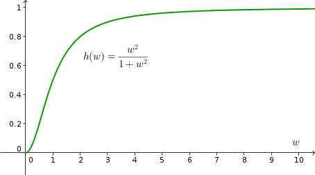
The fact that the predation rate $h(w)$ saturates to the maximum value of 1 has an important consequence: the predators can't eat the budworms fast enough to stop an outbreak. When there is an explosion of the spruce budworm population, the birds will eat the budworms at their maximal rate, but it won't be nearly enough to bring the population size back down. Notice that $h(3)=0.9$, or 90% of the maximum. Once the budworm population size reaches around $w=3$, the bird can't respond to additional population growth by eating much more. If the birds can't bring down a huge population of budworms, how will the outbreak come to an end? Let's see what the model tells us.
Model analysis
Putting the predation rate into the model, the final form of our logistic model with predation is \begin{align} \diff{w}{t} = r w \left(1 - \frac{w}{a}\right) - \frac{w^2}{1+w^2}. \label{logistic_predation} \end{align} This model is much too complicated to have a nice formula for the solution. Instead, we will seek to understand the behavior of the spruce budworm population size $w(t)$ using graphical methods, as well as approximations to the solution using the Forward Euler algorithm.
One challenge is that we don't have values for the parameters $r$ and $a$. This may seem like an inconvenience, but it will turn out that allowing the parameters to take on different values will be key to understanding the behavior of the outbreaks.
To begin, you can explore the behavior of the model using the following applet. In the left panel, you can study the plot of the right hand side of equation \eqref{logistic_predation}, i.e.,
\begin{align*}
f(w) = r w \left(1 - \frac{w}{a}\right) - \frac{w^2}{1+w^2}.
\end{align*}
You can explore how this function depends on the parameters $r$ and $a$.
Spruce budworm model. Illustration of the dynamical system modeling an outbreak of the spruce budworm population. The evolution of the budworm population $w(t)$ is modeled by the autonomous differential equation $\diff{w}{t}=f(w)$, where
\begin{align*}
f(w)= r w \left(1 - \frac{w}{a}\right) - \frac{w^2}{1+w^2}.
\end{align*}
The left panel shows a plot of $f(w)$ (black curve), which changes depending on the value of the parameters $r$ and $b$ (changeable via sliders). If you click the play button in the lower left corner of one of the panels or increase $t$ manually via the red slider in the right panel, the evolution of $w(t)$ from the initial condition $w(t_0)=w_0$ is shown by the blue curves. In the left panel, $w(t)$ is a line on the horizontal axis. In the right panel, $w(t)$ is plotted versus time $t$. The direction of $w(t)$ can be determined by the sign of $f(w)$ or by turning on the vector field (with check box). Equilibria are displayed by circles in the left panel and horizontal lines in the right panel if you check the box.
The build-up toward the insect outbreak
Let's explore some of the key features of the model that will help explain the spruce budworm outbreaks. Set the parameters back to their initial values: $r=0.52$ and $a=3.6$. How many equilibria does the equation have? What are their values? Are they stable or unstable? For each stable equilibrium, determine the initial conditions for which the solution will converge to the equilibrium.
This parameter regime should correspond to a low level of insects. Since the carrying capacity $a$ is small, we could think of the forest as being small. Looking at the above plot of $h(w)$, what is the rate of bird predation when the budworm population is at this stable equilibrium? Have the birds gotten to their maximum predation level? You should see that the birds are eating at a moderate level. The birds are able to keep the budworm population in check.
Now, let's imagine the forest is growing so that the carrying capacity for the budworms increases. As you increase $a$, do you notice any big changes in the graph of $f(w)$? What happens just as you bring $a$ above 7.1 or so? When $a$ is around 7.5, how many equilibria does the equation have? What are their values? Are they stable or unstable? For each stable equilibrium, determine the initial conditions for which the solution will converge to the equilibrium.
In this parameter regime, you should see two stable equilibria. One is at a low budworm population size, pretty close to the one we saw above. But, there is a new stable equilibrium at a larger value of population size $w$. That equilibrium corresponds to the outbreak of spruce budworms. What is $h(w)$ at the upper equilibrium? Have the predators pretty much reached their capacity at this population size?
If we started with a small forest, which means a low spruce budworm population, and the forest then grew to this size ($a$ around 7.5), which equilibrium would you expect the budworm population size to converge to? Would the budworms be at the lower equilibrium where they are controlled by the birds? Or the upper equilibrium corresponding to the outbreak? This question can be resolved from your knowledge about which initial conditions converge to which equilibrium.
If you further increase the forest size to give a carrying capacity around $a=20$, you shouldn't see any qualitative differences from the $a=7.5$ case. What quantitative difference do you observe? In other words, what has changed about the location of the equilibria? If one started with a low spruce budworm population size, would the population size be exploding or would the population size still be kept in check by the predators?
The outbreak
If the situation was precarious when $a=20$, it gets downright ugly when the forest grows much larger and increases the carrying capacity. Something happens to the equilibria when the carrying capacity gets much larger than $a=27$. Describe the situation when the carrying capacity is around $a=30$. How many equilibria does the equation have? What are their values? Are they stable or unstable? For each stable equilibrium, determine the initial conditions for which the solution will converge to the equilibrium.
Don't blindly trust the Forward Euler approximation (blue curve) of the graph. Use the Forward Euler approximation as a guide, but also estimate a solution using a graphical approach based on the graph of $f(w)$. If the blue curve seems to stop where it shouldn't (such as away from an equilibrium), you can try increasing the total time $t_f$ of the simulation to see if you can get the blue curve to behave like you know it should (based on the analysis of the graph of $f(w)$).
When the forest is large enough for the carrying capacity to be around $a=30$ (and the growth rate is fixed at $r=0.52$), you should have discovered that there's no avoiding the population explosion in the spruce budworm. The population skyrockets to nearly $w=30$. There are budworms everywhere, and they are busy eating the leaves off the trees, decimating the forest.
Are the birds doing much to control the situation? What is $h(w)$ for the outbreak equilibrium? Is it much larger than when the budworms population $w$ was a tenth this size? The birds are enjoying their feast, but only putting a small dent into the budworm population size.
The decline of the outbreak
What finally puts an end to the outbreak? What the birds couldn't do, the budworms do to themselves. After a prolonged outbreak, the spruce budworms cause a vast defoliation of the fir and spruce trees. This decreases the amount of food available for the budworms, effectively decreasing the carrying capacity of the forest. If the available food can't support the huge population of budworms, many of them will die of starvation, decreasing the population size. Let's investigate how the model predicts this starvation should end the outbreak.
Imagine that the defoliation due to the budworm outbreak decreased the carrying capacity back down to $a=20$. You don't need to analyze the equilibria for this value of $a$ again; you did all the work already. For these parameters, you should have showed above that the birds could keep the population under control and the outbreak was prevented. Therefore, when the carrying capacity gets back down to $a=20$, the outbreak should be ended, and we should be back to a small population of budworms, right?
Do you agree with that last sentence? If we start with a huge population of budworms and bring the carrying capacity down to $a=20$, which equilibrium should the budworm population size converge to? Is the outbreak still occurring or has it ended?
Assuming you determine that the outbreak is still occurring, then the budworms should continue their defoliation of the trees, dropping the carrying capacity even further. Even when the carrying capacity drops all the way down to $a=7.5$, we still had two stable equilibria. One corresponded to a small population size and one to the outbreak. If the carrying capacity was brought down to $a=7.5$ by feasting budworms, which equilibrium should the system be approaching? Is the outbreak still occurring or has it ended?
Another qualitative change occurs by the time the carrying capacity drops below $a=7$. What is the dramatic difference between the situation when $a$ is around 7.5 and the situation when $a$ is around 6.5? Describe what is different about the equilibria. When a large population brings the carrying capacity down to this level, what must finally happen to the budworm population size?
The idea is that when the carrying capacity gets this low, most of the budworms that don't die from starvation can be taken care of by the birds. The budworms managed to defoliate a large portion of the forest, but have finally been brought down to a small population where they don't do much damage. That is, at least until the forest grows back large enough so that the population can explode again. But that will take 40 or so more years.
A summary figure
To present your results to foresters and folks in the wood products industry, you need a way to nicely summarize your results. One way to do this would be to make a movie using the above applet. You could set the initial condition $w_0$ to a small value and the time $t$ to some large number so that $w$ is always at the lower stable equilibrium. As the forest grows and the carrying capacity $a$ slowly increases, the budworm population size would track the lower stable equilibrium until that equilibrium suddenly disappears, and the population explodes to the upper equilibrium. For the second half of the movie, set the initial condition to a large value so that $w$ is at the upper stable equilibrium. As forest dies and $a$ decreases, the population size stays at the upper equilibrium until that equilibrium suddenly disappears and the population drops back down to low levels.
An example of such a movie is shown below. Click the play button (at lower left of one of panels) to get it started. The right panel plots a graph of the population size versus time. (The $T$ from the movie is slower time scale than the $t$ in the first applet.)
Spruce budworm outbreak movie. This movie illustrates how the spruce budworm population size initially stays low as the forest grows, until finally the population explodes into a outbreak of the budworms which decimates the forest. Click the play button in the lower left corner of one of the panels to start the animation. The left panel shows a plot of $f(w)=rw(1-r/a)-w^2/(1+w^2)$, which is the right hand side of the spruce budworm model $w'(t)=f(w)$. The movie does not show the evolution of this differential equation, but just sets that the budworm size to be a stable equilibrium of the model. (The movie assumes that the evolution to the equilibrium happens faster than the time scale represented.) The right panel shows how the population size $w$ and the carrying capacity $a$ of the forest evolve with time $T$. When the budworm population is low, the forest grows so that the carrying capacity $a$ increases steadily. Then, when the outbreak occurs, the forest dies and the carrying capacity $a$ decreases steadily. The rate of increase and decrease of $a$ is arbitrary; the time $T$ is some slow time scale over which the forest evolves.
You like this movie but realize that you need a simpler way to communicate the results. You decide it would be better to have something just on a piece of paper that you can hand out to people and that allows folks to see the whole situation with just one glance. Your idea is that you could capture the essence of the whole movie with a plot of $w$ versus the carrying capacity $a$.
The crux of the idea is the following. Imagine that you turn off the view of the function (and the vector field) in the first applet and just show the equilibria on the $w$ phase line. The summary figure will just show how the equilibria on the $w$-axis change as you change $a$. Flip the $w$-axis so it becomes the vertical axis. Make the horizontal axis be the $a$-axis. Above each value of $a$, plot the values of the equilibria. Above some values of $a$ (such as $a=3$), you would just plot two circles, corresponding to the positions of the two equilibria. Above other values of $a$ (such as $a=7.5$), you would put four circles. Since the location of the circles change smoothly as you change $a$, the track of the circles would trace out smooth curves as you moved from left to right (moved from small values of $a$ to large values of $a$).
In fact, the plot would be even clear if, rather than plotting the individual circles, you just drew the smooth curves showing how the equilibria change as $a$ changes. You would use solid lines for stable equilibria and dash lines for unstable equilibria. For example, you would have a straight dashed line across the whole diagram at $w=0$, since that unstable equilibrium is there for all values of $a$. The other equilibria move around as you change $a$, so they would be represented by curves. This plot is a bifurcation diagram. Don't use that term in front of the foresters, though, or they may get nervous and get scared of the mathematics.
Once you have created a nice bifurcation diagram representing how the equilibria depends on $a$, the last part is to show the foresters what happens to the spruce worm population $w(t)$. The population size will never approach an unstable equilibria, of course. But, it will stay close to different stable equilibria depending on the situation. Since this diagram doesn't show time, you can draw how $a$ and $w$ evolved in the movie using a curve (a different color?) with arrows on it. The arrows will distinguish when $a$ is increasing and when $a$ is decreasing. If you start at a small value of $a$ and $w$, increase $a$ through the catastrophic outbreak. Then, once $w$ jumps up to the outbreak level, bring $a$ back down until $w$ jumps down to a low level. The curve with arrows representing this sequence of events should trace out a loop, and the curve should be on the stable equilibria from the bifurcation diagram except at the points where it jumps and and down. This loop is how you'll explain the outbreak to the foresters. (It's called a hysteresis loop, but again, keep the fancy lingo to yourself.) The hysteresis loop, when drawn on top of the bifurcation diagram, succinctly tells the story of the above movie in one diagram.
When you make this summary diagram, with $a$ on the horizontal axis and $w$ on the vertical axis, be sure to label everything clearly so the foresters can understand what your model is telling them. You could include labels from the movie, if you like. Use this diagram to tell the story of how the model predicts how the spruce budworm outbreak initiates and is terminated. Remember, the foresters may not understand mathematics very well, so include enough description so that they can follow what you did.
Project
The spruce budworm outbreak project page gives instructions for writing up a project report based on this analysis.
Thread navigation
Elementary dynamical systems
- Previous: Worksheet: Introduction to a bifurcation diagram
- Next: Model of an infectious disease without immunity
Math 1241, Fall 2020
Math 201, Spring 22
Similar pages
- Introduction to bifurcations of a differential equation
- A simple spiking neuron model
- The Forward Euler algorithm for solving an autonomous differential equation
- An introduction to ordinary differential equations
- Exponential growth and decay: a differential equation
- Solving single autonomous differential equations using graphical methods
- Single autonomous differential equation problems
- Two dimensional autonomous differential equation problems
- Solutions to two dimensional autonomous differential equation problems
- Initial dynamical systems exploration
- More similar pages