Initial dynamical systems exploration
Let's explore some basic ideas about a dynamical system, which is a system where things change over time according to some fixed rule. We will use Geogebra to visualize concepts such as the state space of a dynamical system and the rule for the evolution of the state variables.
Evolution of the size of an anteater population
Introduction
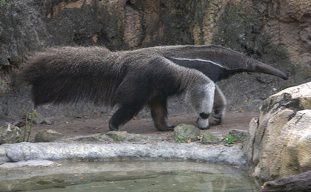
Let's use a dynamical system to model the evolution of the size of a population of anteaters. The first step in defining a dynamical system is to determine the state variable(s), i.e., variables whose values indicate the current state of the system. In this case, we'll assume we can base our model on just the total anteater population size (and not worry about other details such as the the locations or ages of the anteaters). This assumption means we can use a single state variable. Let's denote the state variable by $a$ and define $a$ to be the total number of anteaters in the population. It's clear only non-negative values of $a$ make sense, so the state space will be the set of non-negative numbers, which we can represent by a number line.
The number $a$ of anteaters will change over time as anteaters are born and die. In other words, we have a dynamical system where the state changes. Let's use $t$ to denote time in years. Then we can use the notation $a(t)$ to indicate the value of the state variable $a$ after $t$ years from the time we start modeling the anteater population. We'll use a continuous-time dynamical system, meaning we will let time vary continuously so that $t$ can be any non-negative real number. With this convention, $a(10.1532)=132$ indicates that the anteater population contains 132 anteaters after 10.1532 years from when we started modeling the population.
Exploring the anteater model
The second component of a dynamical system, after definition of the state variables, is the rule for the evolution of the state variables. Since a continuous-time dynamical system requires derivatives, and we don't expect knowledge of derivatives at this point, we won't give the equations for the evolution of our anteater model. Instead, we'll use the below Geogebra applet to explore the behavior of the anteater dynamical system. (If you are familiar with derivatives and would like to see the equation behind the model, you can check out the applet page.)
In the applet's initial state, time is fixed at $t=0$. The left panel shows the state space depicted as a blue number line. This state space is labeled as population size $x(t)$, but we want to use $a$ for our state variable since we are dealing with a population of anteaters. In the box labeled state variable, change the $x$ to an $a$ (and press Enter). All references to the state variable should now be in terms of $a$.
The large blue dot represents the value of the state variable at time $t=0$, i.e., $a(0)$. We call this initial value the initial condition of the dynamical system. We often write the initial condition as \begin{align*} a(0) = a_0, \end{align*} so we can use $a(0)$ and $a_0$ interchangeably. You can change the initial condition by dragging the blue point with your mouse or by typing a new value in the box labeled by $a_0$ (assuming you changed the state variable to $a$). If you left the time at $t=0$, then $a(t)$ is the same as $a_0$ and changes with it. The size of the population of anteaters is also indicated by the green diamonds in the right panel, where each diamond represents one anteater.
Evolution of a bistable population. The evolution of the size $x(t)$ of a population is illustrated in three different ways. In the right panel, each green diamond represents one individual in the population, so the the population size $x(t)$ is given by the number of green diamonds. You can change time $t$ by dragging the red point on the red slider in the left panel or by clicking the triangle in the lower-left corner of one of the panels to start the animation. The state space, or space of possible values of $x(t)$, is represented by the blue line in the left panel. The initial condition $x_0$, or population size at time $t=0$, is shown by the large blue point in the state space. The population size $x(t)$ at time $t$ is shown by the small red point on the state space (visible only if $t > 0$). If you check the “plot versus time” box, then the right panel displays a green curve indicating how the population size changes as a function of time. The height of the blue dot on the curve indicates the initial population size $x_0$ at time $t=0$, and the height of the red dot on the curve indicates $x(t)$ for the time $t$ shown in the left panel. The evolution of the population size shows bistable behavior so that the population size either crashes to zero (i.e., the population dies out) or the population size approaches a larger value (i.e., the population survives). The fate of the population depends on the initial condition $x_0$ (which you can change by typing a value in the box or dragging one of the blue points). You can change the value of the larger population size (and other parameters affecting how the population evolves) by checking the “advanced options” and changing the values of the parameters. You can also change the name of the state variable $x$ to another variable by entering a different letter in the state variable box.
Next, let the population of anteaters evolve. Press the play (triangle) button that is in the lower left corner of one of the two applet panels to start the animation. Then, time $t$ increases steadily up to $t=30$ years before reseting back to zero, as indicated by the red slider. The corresponding value of $a(t)$ is shown by the red point on the blue number line representing the state space, and the number of diamonds changes to match $a(t)$.
What happens to the anteater population as time begins to increase from $t=0$. Does the population begin to increase or decrease, or does it stay at the same size? As more time passes and $t$ approaches 30 years, do the anteaters survive or does the population size drop toward zero? Does the population continue the trend (increasing or decreasing) it had in the beginning, or does it oscillate up and down? Does it grow faster and faster so that the population size explodes or does the population stabilize toward a steady value?
One can determine how the population size evolves by analyzing the movie of $a(t)$ changing with time (represented by either the red point in the left panel or the green diamonds in the right panel). It is easier, though, to analyze a summary plot that captures all values $a(t)$ for the thirty years with $0 \le t \le 30$. To view a plot of population size $a$ versus time $t$, you can click the “plot versus time” checkbox. In the resulting plot (right panel), the state space for $a$ is shown flipped vertically. The blue vertical axis is the same as the blue number line in the left panel for the initial time $t=0$. Hence, you can also change the initial condition $a_0$ by moving the blue point in the right panel up and down. The values of the population size for later times is shown by the green curve. When the animation is playing, a red dot representing $a(t)$ moves steadily to the right along the green curve, in sync with the red point in the left panel. The moving thin blue line represents the state space at time $t$.
With the plot versus time, you can quickly verify your analysis from the movie of $a(t)$. This plot will also help you analyze the dependence of the population behavior on initial condition $a_0$. How does the behavior of the population (and its ultimate fate) depend on the initial population size? As you vary the initial population size, how many different long term outcomes are possible? Can you find initial conditions where the population dies out, explodes to arbitrarily large values, approaches a steady value, or oscillates up and down? (Not all of these options are possible for this model.) For each of these possible outcomes, what is the range of initial conditions that leads to that outcome?
The decay of lead in the bloodstream
Introduction
As lead is a strong poison, small amounts of lead in the body can cause lead poisoning, leading to serious health problems. The body does eliminate lead, such as through urine, but the elimination is slow. Elimination from the bones can take decades, but we'll model how the lead level in the bloodstream decays, which is a faster process.
We can use a simple dynamical system model where the state variable $p$ is the concentration of lead in the blood, measured in μg/dl (micrograms per deciliter). If no further sources of lead are introduced, then lead will be slowly eliminated from the body. Let's imagine that the amount of lead decreases by 11% each week.
Although the lead level changes continuously over time, let's just model weekly snapshots of the lead concentration. (You could imagine that a doctor is testing a patient's lead concentrations each week, and we'll work with just these weekly numbers.) We'll use a discrete-time dynamical system, where the time interval is one week. Let $t$ measure time in weeks, and we'll allow $t$ to take only non-negative integer values. We'll start at $t=0$. The value $t=1$ will represent one week later, $t=2$ will represent two weeks later, etc.
We'll use $p_t$ to denote the lead level at time $t$. We use the notation convention as a subscript for $t$, using $p_t$, because we have a discrete-time dynamical system and $t$ is always an integer. (If we were using a continuous time model, then we would have used $p(t)$ instead, as we did for the anteater population size $a(t)$.) We'll denote the lead level at time $t=0$ (the initial condition) by $p_0$, the lead level after one week by $p_1$, the lead level after two weeks by $p_2$, etc.
Since the lead level decreases by 11% each week, we can write a simple formula for the dynamical rule: the lead level after a week is 89% of the previous lead level. Therefore, the rule for the first week is $p_1=0.89 p_0$, the rule for the second week is $p_2=0.89p_1$, the rule for the third week is $p_3=0.89p_2$, etc. We can summarize all these steps by saying that if the lead level in week $t$ is $p_t$, then the lead level the next week (in week $t+1$) is 0.89 times $p_t$, i.e., \begin{align} p_{t+1} = 0.89 p_t. \label{leaddecay} \end{align}
Obtaining the applet for the lead decay model
To explore the lead decay, we'll use Geogebra again. This time, though, we'll interact with the Geogebra applet in a different way. For the anteater model, we just manipulated the applet embedded in the web page. For the lead model, you'll need more control over the applet, so you'll run Geogebra on your own computer and manipulate the Geogebra construction directly.
The first step is to download and install Geogebra on your computer, if you haven't already. To do so, go to the Geogebra download page. Once you have Geogebra up and running, the next step is to download the below Geogebra applet. To go to the applet page by clicking the “more information about applet” link at the bottom of the applet caption, below. If you scroll down on the applet page, you'll find the applet file, in this case labeled “discrete_dynamical_system_spreadsheet.ggb.” Click the filename and save the file to your computer somewhere. You can open the file from within Geogebra (select Open from the File menu) or double-click the file to launch Geogebra with the file.
Discrete dynamical system with spreadsheet.
When you open the file within Geogebra, it should look like the above applet.
Setting up the applet for the lead decay model
The next step is to use the applet to calculate the evolution of our lead concentration dynamical system of equation \eqref{leaddecay} and create a plot of the results. The following video demonstrates how to use the integration of the Geogebra spreadsheet and Graphics window to create an applet for our model. You can either watch the video or read the rest of the text of this subsection, as they both explain the same procedure.
Using applet to explore lead level decay.
Let's focus on the spreadsheet, which has three columns. Column A is for the time points and column B is for the corresponding value of the state variable $p_t$. (The first column is labeled in cell B1 as $x_t$, but you can change it to $p_t$ if you like: double click cell B1 and change x_t to p_t.)
Column C creates the points $(t,p_t)$, which are displayed in the left panel. (You can change the label in cell C1 from $(t,x_t)$ to $(t,p_t)$ if you like.) Geogebra automatically creates points in the graphics window if you type an ordered pair like (3,2) into a spreadsheet cell. You can experiment by typing an ordered pair into any cell of the spreadsheet. (Select the cell with your mouse and press Delete to get rid of the point.) We'll use this feature to create a plot of how the lead concentration decreases over time.
Our goal is to use this applet to plot the solution to the dynamical system of equation \eqref{leaddecay}. We'll calculate the evolution using column B and use column C to plot the result. The initial condition $p_0$ is in cell B2. Let's imagine that we started with a high level of lead in the blood, say 64 μg/dl, so change the initial condition by typing 64 into cell B2. (The points may disappear in the Graphics window because they are beyond the scale of the vertical axis. You can change the scale of the vertical axis by holding shift and dragging up or down on the axis with your mouse.)
To program the correct dynamical rule of equation \eqref{leaddecay}, we need to change the formula in cell B3. By default, it just adds one to the initial condition in B2; we'll make it multiply B2 by 0.89. Right-click cell B3, click Object Properties. In the Basic tab, change the Definition to be “0.89*B2” and press Enter. With that change, the applet should calculate the value of $$p_1 = 0.89p_0 = 0.89(64) = 56.96$$ in cell B3 and plot the point $(1,56.96)$ in the graphics window. The formula in cell B3 now implements to our rule that the lead level should decay to 89% its previous level after one week. As a result, the lead level should be down to 56.96 μg/dl in week 1.
To evolve the discrete dynamical system, one just needs to keep iterating the rule “multiply by 0.89” to march time forward week by week. We can use the spreadsheet to quickly do this calculation for us. Simply highlight the last row in the table (cells A3, B3, and C3), press Ctrl+C to copy them, click cell A4, and press Ctrl+V to paste. This copies the formulas into cells A4, B4, and C4, so that B4 contains the value \begin{align*} p_2 = 0.89 p_1 = 0.89(56.96) \approx 50.69, \end{align*} and C4 contains the point $(2,p_2)=(2,50.69)$, which is also plotted in the Graphics window.
You can continue this process by pasting the formula into A5. Or, you can paste into many rows at once. However, unlike other spreadsheets, you have to highlight more than just a range of cells in column. Instead, you need to highlight a rectangle of cells in columns A-C and as many rows as you like. Then, press Ctrl+V to paste the formulas into all those rows, and calculate the lead concentration $p_t$ for many time points $t$.
The result should be a list of the values of $p_t$ in column $B$ and sequence of points of concentration versus time point in the Graphics window. Geogebra labels all the points with their spreadsheet cell: C2, C3, C4, etc. We don't want to show those labels, as they are irrelevant for the dynamical system model. To hide the labels, select the points in the Graphics window by dragging a rectangle around them with the mouse, right click a point, and click Show Label to turn off the labels.
To make the plot understandable, we should label it to make the content clear. The horizontal axis represents $t$, which is in weeks. Label it “time t (weeks)” by clicking the Graphics Window, clicking the ![]() Insert Text Tool, clicking where you want the text, then entering the text in the dialog box that appears. The vertical axis represents the lead concentration $p_t$; label it “lead level p_t (μg/dl),” where you can get the μ from clicking the Symbols button and looking in the Basic section. This long label for the vertical axis should be rotated, but it's complicated to get rotated text, Greek symbols, and superscripts together in Geogebra. Instead, you can just press Enter between words to space the words out vertically.
Insert Text Tool, clicking where you want the text, then entering the text in the dialog box that appears. The vertical axis represents the lead concentration $p_t$; label it “lead level p_t (μg/dl),” where you can get the μ from clicking the Symbols button and looking in the Basic section. This long label for the vertical axis should be rotated, but it's complicated to get rotated text, Greek symbols, and superscripts together in Geogebra. Instead, you can just press Enter between words to space the words out vertically.
Geogebra makes it easy to change the symbols or colors used in the plot. Just right click an object, select Object Properties, and take a look around.
Exploring the lead decay model
Since the applet is doing all the calculations, you are free to look at the big picture to understand the dynamics of the elimination of lead from the bloodstream. In particular, you can determine how fast the lead is eliminated as predicted from the model. About how long does it take for the lead concentration to drop down to half its original concentration? One quarter? One eighth? How does the time required to drop to these levels depend on the initial lead level $p_0$? For example, does it seem like it will take longer for the lead level to drop to half of $p_0$ if you increase $p_0$ above 64 μg/dl or if you decrease $p_0$ below 64 μg/dl?
Thread navigation
Math 1241, Fall 2020
Math 201, Spring 22
Similar pages
- Spruce budworm outbreak model
- A simple spiking neuron model
- Equilibria in discrete dynamical systems
- The idea of stability of equilibria for discrete dynamical systems
- Discrete dynamical systems as function iteration
- Solving linear discrete dynamical systems
- More details on solving linear discrete dynamical systems
- A graphical approach to finding equilibria of discrete dynamical systems
- The idea of a dynamical system
- An introduction to discrete dynamical systems
- More similar pages