Calculating the area under a curve using Riemann sums
The area under a curve
Given a function $f(x)$ where $f(x) \ge 0$ over an interval $a \le x \le b$, we investigate the area of the region that is under the graph of $f(x)$ and above the interval $[a, b]$ on the $x$-axis. For example, the below purple shaded region is the region above the interval $[-1,10]$ and under the graph of a function $f$. Such an area is often referred to as the “area under a curve.”

Since the region under the curve has such a strange shape, calculating its area is too difficult. But calculating the area of rectangles is simple. Let's simplify our life by pretending the region is composed of a bunch of rectangles. To turn the region into rectangles, we'll use a similar strategy as we did to use Forward Euler to solve pure-time differential equations.
As illustrated in the following figure, we divide the interval $[a,b]$ into $n$ subintervals of length $\Delta x$ (where $\Delta x$ must be $(b-a)/n$). We label the endpoints of the subintervals by $x_0$, $x_1$, etc., so that the leftmost point is $a=x_0$ and the rightmost point is $b=x_n$. The picture shows the case with four subintervals.
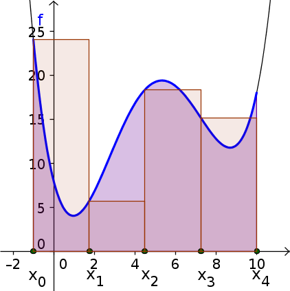
The next step is to pretend that $f(x)$ doesn't change over each subinterval. We'll measure $f(x)$ on the left side of the subinterval, and ignore any changes in $f$ across the subinterval. The result is that we are pretending that the region under $f$ is composed of a bunch of rectangles, one for each subinterval. Maybe it's a crude approximation, but it makes for an easy calculation of area.
Let's number the $n$ subintervals by $i=0,1,2, \ldots, n-1$. Then, the left endpoint of subinterval number $i$ is $x_i$ and its right endpoint is $x_{i+1}$. We are imagining that the height of $f$ over the entire subinterval is $f(x_{i})$, the value of $f$ at the left endpoint. Since the width of the rectangle is $\Delta x$, its area is $f(x_{i})\Delta x$.
To estimate the area under the graph of $f$ with this approximation, we just need to add up the areas of all the rectangles. Using summation notation, the sum of the areas of all $n$ rectangles for $i=0, 1, \ldots, n-1$ is \begin{align} \text{Area of rectangles} = \sum_{i=0}^{n-1} f(x_{i}) \Delta x. \label{left_riemann} \end{align} This sum is called a Riemann sum.
The Riemann sum is only an approximation to the actual area underneath the graph of $f$. To make the approximation better, we can increase the number of subintervals $n$, which makes the subinterval width $\Delta x= (b-a)/n$ decrease. To explore what happens as $n$ gets larger and larger, you can use the following applet.
Area via a left Riemann sum. The area underneath the graph of $f(x)$ (blue curve in left panel) over the interval $[a,b]$ is calculated via a left Riemann sum. The left Riemann sum of $n$ subintervals is illustrated by the rectangles superimposed with the graph of $f$. The right panel shows the area of the rectangles $\hat{A}(x)$ from $a$ to $x$, plotted as a green curve. The area over the whole interval $[a,b]$ is the value $\hat{A}(b)$. To investigate the behavior of $\hat{A}$, you can move pink points along the curve and the tops of the rectangles. As you move the pink points, a rectangle is highlighted, and the calculation of its area is shown in the upper right corner. The area of each rectangle is the value of $f$ at its left endpoint times the subinterval width $\Delta x$. The running sum of the area, $\hat{A}(x)$, increases by the area of a rectangle when you move the pink points right one rectangle. If you check the “exact” box, the true area under the graph of $f$ is shaded in red at the left and the right panel displays a graph (in red) of the true area $A(x)$ under $f$ from $a$ to $x$. The true area through the right of the highlighted rectangle is calculated along with the error between the true area and the corresponding area calculated with the Riemann sum. The values of $A(x)$ and $\hat{A}(x)$ are areas under $f$ only for the case when $f(x) \ge 0$.
For $f(x)=x^3/3-2x^2+12$, write out all four terms of the Riemann sum with $n=4$ that estimates the area underneath the graph of $f$ over the interval $[a,b]=[-2,7]$. Plug in the numbers from $f$ evaluated at the left endpoints, and calculate this estimate of the area. This estimate should agree with what you calculate with the above applet for that function and four subintervals.
What happens as you increase $n$ further and further? If you divide the interval $[-2,7]$ into 100 subintervals of length $\Delta x = 0.09$, what is the estimate of the area under the graph of $f$? How about for $n=1000$ and $\Delta x=0.009$? Do the estimates for the area seem to converge as $n$ increases? To look at this convergence, check if the the estimates change less and less as you keep doubling the number $n$ of subintervals.
The definite integral
As we let $n$ get larger and larger (and $\Delta x$ smaller and smaller), the value of the Riemann sum \eqref{left_riemann} should approach a single number. This single number is called the definite integral of $f$ from $a$ to $b$. We write the definite integral as \begin{align*} \int_a^b f(x)dx &= \lim_{n \to \infty} \sum_{i=0}^{n-1} f(x_{i}) \Delta x. \end{align*} The integral sign $\int$ refers to a sum just like summation sign $\sum$. (OK, it's a sum over an infinite number of terms, whatever that means, but let's not get hung up on that.) When we integrate a function $f$ from $a$ to $b$, we are just adding up values of $f(x)$ for $x$ going from $a$ to $b$.
Another important thing to remember is that the definite integral $\int_a^bf(x)dx$ is just a single number. This fact is in contrast to the indefinite integral $\int f(x)dx$, which, although it looks similar, is something different. The indefinite integral $\int f(x)dx$ is a function (actually a whole family of functions, as you can add an arbitrary constant). When you add the limits of integration $a$ and $b$, the expression turns into a definite integral $\int_a^b f(x)dx$, which is just a number. In this case, we are viewing the number as the area under the function $f$ over the interval $[a,b]$.
Right sum
So far, we built our Riemann sum \eqref{left_riemann} by using rectangles whose height was equal to $f$ evaluated at the left endpoint of each subinterval. We call this Riemann sum a left Riemann sum. What if we used the value of $f$ at the right endpoint rather than the left endpoint? The result is the right Riemann sum \begin{align} \text{Area of rectangles} = \sum_{i=0}^{n-1} f(x_{i+1}) \Delta x. \label{right_riemann} \end{align} The only difference from the left Riemann sum \eqref{left_riemann} is that we evaluate $f$ in interval $i$ at the right endpoint $x_{i+1}$.
Since $f$ actually does change over the course of the subinterval, we expect that the left Riemann sum will give a different area than the right Riemann sum. How does the right Riemann sum compare to the left Riemann sum? The below applet will let you experiment. As you make the number of interval $n$ larger, does the estimate of the area converge to a single number? Does this number seem to be the same as with the left Riemann sum?
Area via a right Riemann sum. The area underneath the graph of $f(x)$ (blue curve in left panel) over the interval $[a,b]$ is calculated via a right Riemann sum. The right Riemann sum of $n$ subintervals is illustrated by the rectangles superimposed with the graph of $f$. The right panel shows the area of the rectangles $\hat{A}(x)$ from $a$ to $x$, plotted as a green curve. The area over the whole interval $[a,b]$ is the value $\hat{A}(b)$. To investigate the behavior of $\hat{A}$, you can move pink points along the curve and the tops of the rectangles. As you move the pink points, a rectangle is highlighted, and the calculation of its area is shown in the upper right corner. The area of each rectangle is the value of $f$ at its right endpoint times the subinterval width $\Delta x$. The running sum of the area, $\hat{A}(x)$, increases by the area of a rectangle when you move the pink points right one rectangle. If you check the “exact” box, the true area under the graph of $f$ is shaded in red at the left and the right panel displays a graph (in red) of the true area $A(x)$ under $f$ from $a$ to $x$. The true area through the right of the highlighted rectangle is calculated along with the error between the true area and the corresponding area calculated with the Riemann sum. The values of $A(x)$ and $\hat{A}(x)$ are areas under $f$ only for the case when $f(x) \ge 0$.
In fact, you should get close to the same number as $n$ gets large. As long as $f$ is nice enough (for example, continuous, or even continuous at all but a finite number of points), these left and right Riemann sums will converge to the same number, which is the definite integral $\int_a^b f(x)dx$.
Forward Euler and area
This method for computing area should seem familiar. It should remind you of how we used Forward Euler to solve pure time differential equations. To make the connection even clearer, let's change our variable name from $x$ to $t$. (The variable name doesn't matter, after all, and $t$ makes more sense so we can talk about time. ) Then, our definite integral is $\int_a^bf(t)dt$ and the corresponding indefinite integral is $\int f(t)dt$.
To make our Forward Euler result be similar to the area estimation problem, let's use $A(t)$ for the variable in a pure-time differential equation, writing it as $\diff{A}{t}=f(t)$. If we make the initial condition be $A(a)=0$, then Forward Euler approximates the solution $A(t)$, i.e., the antiderivative $A(t)=\int f(t)dt$ that has $A(a)=0$. By comparing the sum we wrote for Forward Euler (equation (8) from the Forward Euler page) and the left Riemann sum \eqref{left_riemann}, we should be able to convince ourselves that they are the same when the initial condition is zero.
To emphasize this correspondence between the Forward Euler approximation and the left Riemann sum for area, we made the Forward Euler applets and the area applets in a similar manner. For the area applets, we used rectangles to estimate the definite integral $\int_a^bf(t)dt$. But if you relabel some variables, then the calculation is essentially the same as the Forward Euler calculation. Below, we made an applet that you can transform between the area calculation case and the Forward Euler case that we hope will make the parallel clear.
The Euler algorithm or approximating area with a Riemann sum. Demonstration of the link between the Euler approximation to a pure-time differential equation and calculating the area under a curve. When the “area” box is checked, the area underneath the graph of $f(t)$ (blue curve in left panel) over the interval $[a,b]$ is calculated via a Riemann sum. The Riemann sum of $n$ subintervals is illustrated by the rectangles superimposed with the graph of $f$. As you move the pink points, the region of the rectangles to the left is highlighted, and this area $\hat{A}(t)$ is plotted as a function of $t$ by the green curve in the right panel. When “area” box is unchecked, the solution to the pure-time differential equation $\diff{A}{t}=f(t)$ via the Euler algorithm is illustrated. Only the tops of the rectangles remain, which form an approximation to $f$ that is constant along each subinterval. The green curve in the right panel remains, but its interpretation is an approximation solution to the differential equation where the slope is held constant on each subinterval. This slope is illustrated by the gray lines: constant at the slope in the left panel and a tangent line in the right panel. Unlike for the area calculation, an initial condition $A(a)$ can be changed by dragging the blue point in the right panel or typing a value in the box. In either mode, calculations for $\hat{A}(t)$ for the current subinterval are shown, as well as the exact solution and corresponding error when the “exact” box is checked. The exact solution is also shown by the red curve, and, for the area case, by red shading of the area underneath $f(t)$.
One important difference between the Forward Euler calculation and the area calculation is the initial condition. For the area calculation, we add up area starting with $A(a)=0$. With Forward Euler, we can have an arbitrary initial condition $A(a)$, which you can change only when you uncheck the “area” option in the applet.
To calculate the area under the curve, is it essential that we keep $A(a)=0$? Or, if we let $A(a)$ be another value, can we still estimate the area from the result? Using a different value of $A(a)$ for the Forward Euler calculation means that it estimates a different antiderivative (since the initial condition determines the arbitrary constant). How do we get the area of the region under the graph of $f$ regardless of which antiderivative we use?
The answer lies by comparing the Forward Euler solution to the area solution. We can rewrite equation (8) from the Forward Euler page in the notation used for this page: \begin{align} A(b) &\approx A(a) + \sum_{i=0}^{n-1}f(t_i)\Delta t. \label{fe_sum} \end{align} Take this equation, let $n$ go to infinity to rewrite the equation in terms of the definite integral of $f$ that is the area under the curve. From this, determine how one can determine the area from an estimate of $A(b)$ using Forward Euler with any initial condition $A(a)$. You should test that your method works by trying different values using the applet.
Area of negative functions?
When using the Riemann sums to calculate area, the mathematical formulas still make sense even if $f$ is negative. Negative values shouldn't be a problem since we've shown the calculation is the same as using Forward Euler. When working with Forward Euler, having a negative function wasn't a problem.
If $f$ goes negative, though, will the definite integral still give area? One hypothesis is that the definite integral gives the area under the curve (above the $x$-axis) when $f$ is positive plus the area over the curve (under the $x$-axis) when $f$ is negative. This hypothesis is that the integral $\int_a^b f(x)dx$ would add up both the green areas and the red areas in the following figure. We'll call this sum the “total area.”
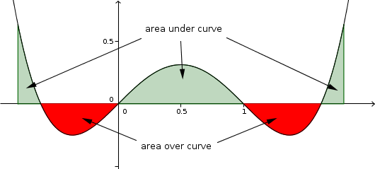
By changing the function in the applet so that it is both positive and negative (or even negative everywhere) in the interval $[a,b]$, test this hypothesis that the integral gives the total area. Does the hypothesis seem to be holding true? If not, what is the relationship between the definite integral $\int_a^b f(x)dx$ and area above or below the graph of $f$? Does this make sense given the definition of the definite integral in terms of a Riemann sum? Remember, the integral is just a sum. What is it adding up here?
If you disagree with the hypothesis that the definite integral $\int_a^b f(x)dx$ gives total area even if $f$ is negative, can you come up with a way to get this total area from a definite integral?
Summary of questions
To aid you in writing up a report on your results, we summarize the main questions posed above that you should be able to answer and added a few more questions.
The area under a curve
- For $f(x)=x^3/3-2x^2+12$, write out all four terms of the Riemann sum with $n=4$ that estimates the area underneath the graph of $f$ over the interval $[a,b]=[-2,7]$. Plug in the numbers from $f$ evaluated at the left endpoints, and calculate this estimate of the area.
- What happens as you increase $n$ further and further? If you divide the interval $[-2,7]$ into 100 subintervals of length $\Delta x = 0.09$, what is the estimate of the area under the graph of $f$? How about for $n=1000$ and $\Delta x=0.009$?
- Do the estimates for the area seem to converge as $n$ increases? To look at this convergence, check if the the estimates change less and less as you keep doubling the number $n$ of subintervals.
The definite integral
- When you calculate a definite integral such as $\int_a^b f(x)dx$, what kind of object should you end up with? A function or something simpler?
- How do this contrast with the indefinite integral $\int f(x) dx$?
Right sum
- Show that the right Riemann sum gives different estimates of the area for small values of $n$, such as for the $n=4$ case you calculated above.
- As you make the number of interval $n$ larger, does the estimate of the area converge to a single number? Does this number seem to be the same as with the left Riemann sum?
Forward Euler and area
- Starting with the sum of equation \eqref{fe_sum} for Forward Euler, let $n$ go to infinity to rewrite the equation in terms of the definite integral of $f$ that is the area under the curve.
- Use this result to determine the expression for how we can determine area even if the initial condition $A(a)$ is not zero. In other words, we want an equation that gives the area (the definite integral) in terms of values of $A(t)$ that works even if $A(a) \ne 0$.
Area of negative functions?
- Does the hypothesis that the definite integral gives total area holding true? If not, what is the relationship between the definite integral $\int_a^b f(x)dx$ and area above or below the graph of $f$?
- Does this make sense given the definition of the definite integral in terms of a Riemann sum? What is the integral adding up?
- If you disagree with the hypothesis that the definite integral $\int_a^b f(x)dx$ gives total area even if $f$ is negative, can you come up with a way to get this total area from a definite integral?
Thread navigation
Math 1241, Fall 2020
Math 201, Spring 22
Similar pages
- Area and definite integrals
- Using the Forward Euler algorithm to solve pure-time differential equations
- Elementary integral problems
- Solutions to elementary integral problems
- Double integrals as area
- Using Green's theorem to find area
- Area calculation for changing variables in double integrals
- Surface area of parametrized surfaces
- Calculation of the surface area of a parametrized surface
- Parametrized surface area example
- More similar pages