Surface area of parametrized surfaces
The calculation of the surface area of a parametrized surface closely mirrors the calculation of the arc length of a parametrized curve. We estimated the arc length of a parametrized curve by chopping up its domain $[a,b]$ into small segments and approximating the corresponding segments of the curve as straight line segments. We could easily calculate the length of the straight line segment approximation to the curve, from which we derived the integral giving the arc length of the curve.
The procedure for calculating surface area is similar. A function $\dlsp: \R^2 \to \R^3$ (confused?) maps a region $\dlr$ in the plane onto a surface. For example, the function \begin{align*} \dlsp(\spfv,\spsv) = (\spfv\cos \spsv, \spfv\sin \spsv, \spsv). \end{align*} parametrizes a helicoid for $(\spfv,\spsv) \in \dlr = [0,1] \times [0, 2\pi]$. Similar to the arc length calculation, the first step in estimating surface area is to chop up the region $\dlr$ into a bunch of small rectangles, as illustrated below.
Applet loading
Applet loading
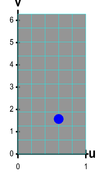
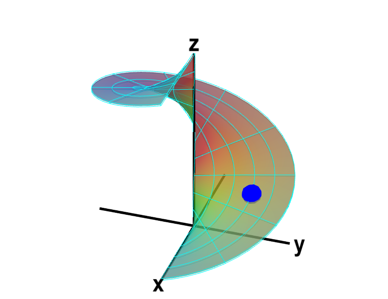
A parametrized helicoid. The function $\dlsp(\spfv,\spsv) = (\spfv\cos \spsv, \spfv\sin \spsv, \spsv)$ parametrizes a helicoid when $(\spfv,\spsv) \in \dlr$, where $\dlr$ is the rectangle $[0,1] \times [0, 2\pi]$. The region $\dlr$, shown as the rectangle in the first panel. You can drag the blue point in $\dlr$ to specify both $\spfv$ and $\spsv$. Alternatively, you can drag the corresponding blue point on the surface in the second panel. In either case, the blue points stay synchronized so that when the blue point in $D$ is at the location $(\spfv, \spsv)$, the blue point on the surface will be at the location $\dlsp(\spfv,\spsv)$.
The region $D$ is divided into small rectangles which are mapped to “curvy rectangles” on the surface. You can click any of the borders of the small rectangles to highlight a curve where one of the variables is constant. Vertical lines in the rectangle $\dlr$ represent curves where $\spfv$ is constant; these correspond to curves that spiral up the helicoid. Horizontal lines in the rectangle $\dlr$ represent curves where $\spsv$ is constant; these correspond to lines that cut across the helicoid. Notice if you drag a blue point along one of these curves, the corresponding blue point in the other panel moves along the corresponding curve. If, for example, you drag the first blue point along the bottom of the rectangle, you change $\spfv$ while leaving $\spsv=0$, and the second blue point moves along the bottom of the helicoid. Similarly, if you drag the blue point along the right side of the rectangle, you change $\spsv$ while leaving $\spfv=1$, and the second blue point spirals around the edge of the helicoid.
The small rectangles form a grid on $\dlr$. The rectangles are mapped by $\dlsp$ onto the helicoid, forming a grid on the surface. In fact, the grid on the surface was shown in all the helicoid applets because we just display an approximation to the true helicoid using such a grid.
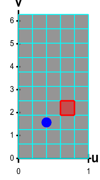
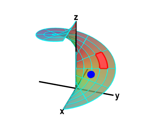
The function $\dlsp$ maps each small rectangle in $\dlr$ onto the surface. Below, you can see below how each rectangle in $\dlr$ (outlined in green) maps onto a small part of the surface, called the image of the rectangle (outlined in red).
Applet loading
Applet loading
A parametrized helicoid with surface area elements. The function $\dlsp(\spfv,\spsv) = (\spfv\cos \spsv, \spfv\sin \spsv, \spsv)$ parametrizes a helicoid when $(\spfv,\spsv) \in \dlr$, where $\dlr$ is the rectangle $[0,1] \times [0, 2\pi]$. The region $\dlr$, shown as the rectangle on the left, is divided into small rectangles, which are mapped onto “curvy rectangles” on the surface at the right. To visualize the mapping, you can click on a rectangle in either panel to highlight it in red; the corresponding rectangle in the opposite panel is also hightlighted in red. The area of the red region on the helicoid depends on how $\dlsp$ stretches or shrinks the small red rectangle of $\dlr$ as it maps it on the surface. You can also drag the blue point in either $\dlr$ or the helicoid surface, and the blue point in the opposite panel moves so that the location of the right point is $\dlsp(\spfv,\spsv)$ when the location of the left point is $(\spfv,\spsv)$.
In reality, the image of each rectangle is some “curvy rectangle” on the surface. (In the above applets, the image of each rectangle appears to have straight edges, but what is shown is only an approximation of the actual helicoid.)
The next step to calculate the surface area is to estimate the area of each of the curvy rectangles. We use exactly the same procedure we did to calculate the “area expansion factor” for a change of variables in double integrals. (In fact, the change of variable function $\cvarf: \R^2 \to \R^2$ can be viewed as a special case of the function $\dlsp: \R^2 \to \R^3$; the surface that $\cvarf$ parametrizes just happens to lie in the plane.)
Let the size of each small rectangle in $\dlr$ be $\Delta\spfv \times \Delta\spsv$. As with changing variables, we approximate each curvy rectangle as a parallelogram spanned by the vectors $\pdiff{\dlsp}{\spfv}\Delta\spfv$ and $\pdiff{\dlsp}{\spsv}\Delta\spsv$. The area of the parallelogram is simply the magnitude of the cross product of those two vectors $$\Delta A= \left\| \pdiff{\dlsp}{\spfv} \times \pdiff{\dlsp}{\spsv}\right\|\Delta\spfv \Delta\spsv.$$
The total surface area is approximated by a Riemann sum of such terms. If we let the rectangles shrink so that $\Delta\spfv$ and $\Delta\spsv$ go to zero, we would see that the total surface area is the double integral \begin{align*} A = \iint_\dlr \left\| \pdiff{\dlsp}{\spfv}(\spfv,\spsv) \times \pdiff{\dlsp}{\spsv}(\spfv,\spsv) \right\| d\spfv\,d\spsv. \end{align*}
The expression for surface area is also similar to the expression we derived for the length of a parametrized curve, \begin{align*} L=\int_a^b \| \dllp\,'(t) \| dt. \end{align*} For surface area, instead of integrating over an interval $[a,b]$, we integrate over the region $\dlr$. In the formula for path length, the expression $\| \dllp\,'(t) \|$ estimates how much $\dllp$ is stretching the interval $[a,b]$ as it maps $[a,b]$ onto the path (or, we could think of it as determining how fast a particle with position $\dllp(t)$ is moving). The expression \begin{align*} \left\| \pdiff{\dlsp}{\spfv}(\spfv,\spsv) \times \pdiff{\dlsp}{\spsv}(\spfv,\spsv) \right\| \end{align*} is analogous to $\| \dllp\,'(t) \|$. It indicates how much $\dlsp$ is stretching $\dlr$ as it maps $\dlr$ onto the surface.
You can read an example here.
Thread navigation
Multivariable calculus
- Previous: A Möbius strip is not orientable
- Next: Calculation of the surface area of a parametrized surface
Math 2374
Notation systems
Similar pages
- An introduction to parametrized surfaces
- Calculation of the surface area of a parametrized surface
- Parametrized surface area example
- Orienting surfaces
- Parametrized surface examples
- Normal vector of parametrized surfaces
- A Möbius strip is not orientable
- Parametrization of a line
- Parametrization of a line examples
- An introduction to parametrized curves
- More similar pages