Discrete dynamical systems as function iteration
A discrete dynamical system models the evolution of state variables of the system over discrete time steps. We imagine that we take a snapshot of the state variables at a sequence of times. The dynamical system model describes a rule for how to evolve from one snapshot to the next.
The simplest case
In the simplest case of a discrete dynamical system, the state space consists of just one state variable, which we'll denote by $x$. For this type of system, all the snapshots mentioned above are just records of the value of $x$ at different times. In this simplest case, the rule for time evolution is also exceedingly simple. The value of $x$ at each snapshot depends just on the value of the previous snapshot of $x$. This value isn't influenced by the actual time of the snapshot, or any earlier values of $x$. If I look at what $x$ is in any given snapshot, I have enough information (given the rule) to know exactly the value of $x$ in the next snapshot.
Since the times of the snapshots don't matter, let's label the sequence of times by integers, so that the snapshots occur at times $t=0,1,2,3, \ldots.$ We'll denote the value of $x$ in the snapshot at time $t=n$ by $x_n$, so the sequence of snapshots is $x_0,x_1,x_2,x_3, \ldots.$ The simple evolution rule for producing this sequence must involve a process that determines each snapshot $x_n$ by looking just at the previous snapshot $x_{n-1}$.
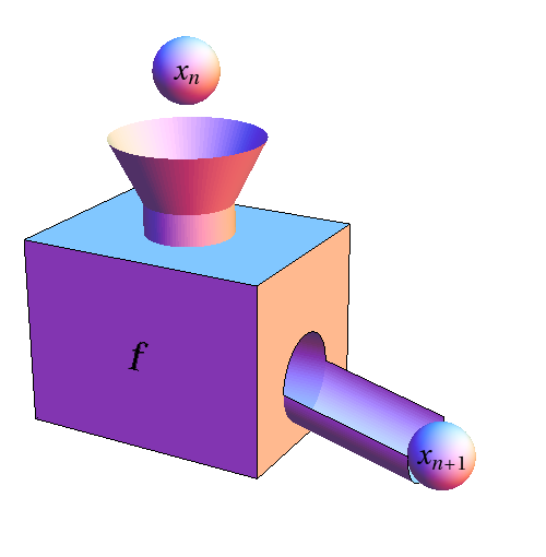
The evolution rule therefore requires a machine that takes in one snapshot as the input and produces the next snapshot. In other words, the evolution rule must be based on a function, which is well described as a function machine, that takes the snapshot $x_n$ at time $t=n$ and produces the next snapshot $x_{n+1}$ at time $t=n+1$.
Let's denote the function that gives the next snapshot by $f$. Then, the evolution rule can be written simply as \begin{gather} x_{n+1} = f(x_{n}) \quad \text{for $x=0,1,2,3, \ldots.$} \label{recursion}\tag{1} \end{gather} Using the function machine metaphor, our evolution rule looks like the following figure, where the snapshots are represented by spheres.
To get the dynamical system going, we have to specify the initial conditions, meaning the state variable $x_0$ at time $t=0$. Given the initial snapshot $x_0$ and the rule $f$, we have now determined all the future snapshots. The snapshot $x_1$ at time $t=1$ is the result of appling $f$ to the initial conditions, \begin{gather*} x_1 = f(x_0). \end{gather*} The snapshot $x_2$ at time $t=2$ is the result of applying $f$ to the snapshot $x_1$ at time $t_1$, which is equivalent to applying $f$ to the initial condition, then sticking the result back into $f$ for a second pass through the function machine, \begin{gather*} x_2 = f(x_1) = f(f(x_0)). \end{gather*}
We can continue this process: \begin{align*} x_3 &= f(x_2) = f(f(x_1))=f(f(f(x_0)))\\ x_4 &= f(x_3) = f(f(x_2))=f(f(f(x_1)))=f(f(f(f(x_0)))). \end{align*} It's a pretty simple process, but writing it out like this gets a bit messy. That's why it easiest to just leave it in terms of the original rule of equation \eqref{recursion}. Equation \eqref{recursion} captures all the steps of the process. We can call it a recurrence relation because it tells us to keep applying $f$ over and over again recursively, using the previous output as the next input.
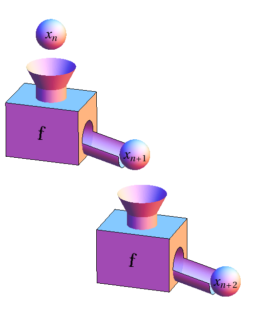
The process of using the output of a function as the input of another function is called composing functions. Function composition is well illustrated by function machines. The following figure shows that if we start with the snapshot $x_n$ at time $t=n$ and apply $f$ twice, we get the result $x_{n+2}$ for two time steps later, at time $t=n+2$. The whole process of evolving this discrete dynamical system could be visualized as a huge chain of these identical function machines hooked together. Since we are composing the same function over and over again, the process is often called function iteration.
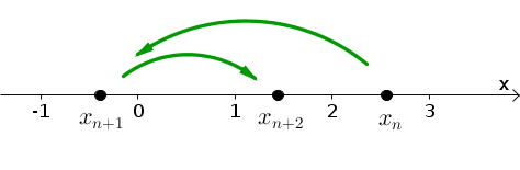
This simple case seems pretty straightforward. Since we have only one state variable, we have a one-dimensional state space, which we can view as just a number line. The state $x_n$ at time $t=n$ is just a point the number line. At the next time step, the point just jumps to a new position $x_{n+1}$.
The following applet lets you explore this function iteration to obtain the sequence of snapshots $x_n$ for a discrete dynamical system. You can specify the two ingredients, the function $f$ and the initial condition $x_0$, and then iterate the function to produce the resulting sequence of snapshots $x_1,x_2,x_3,\ldots$ or the trajectory of the initial point $x_0$. In this applet, we've turned things around a bit, as we are plotting the state space for the snapshots $x_n$ as the vertical axis (which we've highlighted in blue to stress that's where all the action is taking place). We've reserved the horizontal axis to represent time $t$. As you iterate the function and the point jumps around the vertical state space, the temporal sequence of these jumps is illustrated with a plot of the points $(n,x_n)$ in the left panel and a list of these points in the right panel.
Function iteration. The effect of repeatedly applying the function $f(x)$ to the starting value $x_0$ is shown both by the list at the right and the graph at the left. At first, only the initial value $x_0$ is shown in the list and just the point $(0,x_0)$ is shown on the graph. (In the list heading, $x_n$ is written as x_n.) Each time you click the “iterate” button, the function is iterated by applying $f$ to the previous value, using the recursion $x_n = f(x_{n-1})$. Then, the new iterate $x_n$ appears in the list and the new point $(n,x_n)$ appears on the graph. Note that the iteration number $n$ is plotted on the horizontal axis (what you may normally think of as the $x$-axis), and the values of $x_{n}$ are plotted on the vertical axis (what you may normally think of as the $y$-axis). The values of each $x_{n}$ are also marked with horizontal lines and the last value $x_{n}$ is labeled. You can change the function $f(x)$ by typing a new function in the box. You can change the initial point $x_0$ by typing a new value in the box or dragging the blue point. You can zoom the vertical axis with the + and - buttons and pan up and down with the buttons labeled by arrows.
Although a discrete dynamical systems in one variable may seem simplistic, it turns out that these systems are surprisingly mathematically rich. One-dimensional discrete dynamical systems can exhibit a large variety of dynamical behavior. We can easily create systems that demonstrate the following behaviors.
- Simple evolution to a fixed point: use the default function $f(x)=1+0.8x$ in the above applet.
- Blow up: set $f(x)=2x$ to get the bacteria doubling system discussed here.
- Periodic orbits: try $f(x)=1-0.8x^2$, or for a more complicated periodic orbit, try $f(x)=3.55x(1-x)$.
- Chaos: try $f(x)=4x(1-x)$ and change the initial conditions $x_0$.
Extensions to the simplest case
Dependence on actual time
One possible way to extend the simplest case is to allow the evolution to depend on the time as well as the state variable. For example, the dynamics might be influenced by something that depends on time day, such as the amount of light, by something that depends on the time of year, such as average temperature, or by some external force that varies with time. In this case, the actual time of the snapshots might matter, so let's denote the time of the $n$th snapshot by $t_n$. Then, the state variable at the next snapshot could depend not only on the previous value of the state variable $x_n$ but also on the time $t_n$ and equation \eqref{recursion} would be replaced by \begin{gather*} x_{n+1} = f(x_n,t_n) \quad \text{for $x=0,1,2,3, \ldots,$} \end{gather*} where the function $f(x,t)$ depends on both state $x$ and time $t$.
Dependence on more snapshots
Another extension to the model is to allow the evolution to depend not only on the current state but also on the state of some previous snapshots. For example, imagine that $x_n$ represented the number of individuals in a population of some species and that individuals couldn't reproduce until they were one time step old. Then, the evolution of the population at time $t=n$ would depend not only on the current population size $x_n$ but also on the population size $x_{n-1}$ of the previous time step $t=n-1$, as $x_{n-1}$ represents those that were at least one time step old at time $t=n$ and could reproduce. In this case, the recurrence relation \eqref{recursion} would be of the form \begin{gather*} x_{n+1} = f(x_{n},x_{n-1}) \quad \text{for $x=1,2,3,4, \ldots,$} \end{gather*} where $f(x,y)$ is a function that depends on two inputs.
Higher dimensions
In all the above cases, each snapshot was just a single number $x_n$. A discrete dynamical system may be based on additional state variables that evolve together in time and whose dynamics are interrelated. For example, in a predator-prey system, one variable may describe the population size of the predator and the other may describe the prey. If the snapshot at time $t=n$ consists of two variables $x_n$ and $y_n$, the discrete dynamical system may have the form \begin{align*} x_{n+1} &= f(x_{n},y_{n})\\ y_{n+1} &= g(x_{n},y_{n}) \quad \text{for $x=0,1,2,3, \ldots,$} \end{align*} where the functions $f(x,y)$ and $g(x,y)$ determine how the two components evolve through the two-dimensional state space together.
Thread navigation
Math 1241, Fall 2020
- Previous: Problem set: Discrete dynamical system introduction
- Next: Introduction to an infectious disease model
Math 201, Spring 22
Similar pages
- Spruce budworm outbreak model
- Equilibria in discrete dynamical systems
- The idea of stability of equilibria for discrete dynamical systems
- A simple spiking neuron model
- Initial dynamical systems exploration
- Solving linear discrete dynamical systems
- More details on solving linear discrete dynamical systems
- A graphical approach to finding equilibria of discrete dynamical systems
- The idea of a dynamical system
- An introduction to discrete dynamical systems
- More similar pages