Math Insight

1. To keep the math simple, we will ignore the three-dimensional nature of the cell. In reality, we would be interested, for example, in how long it would a molecule to diffuse in three dimensions from the edge of the cell (the cell membrane) to somewhere in the center of the cell. Instead, we'll model one-dimensional diffusion across an interval.

   Let's imagine that the molecule is diffusing from the edge of the cell to some location a distance $L$ away. When the molecule reaches that location, it is immediately removed (for example, it could be metabolized into another product). In the one-dimensional model, we'll let $x=0$ represent the edge of the cell and $x=L$ represent the final location near the center of the cell. (The length $L$ could represent the radius of the cell.) We are interested in how long it would take a molecule to diffuse from $x=0$ to $x=L$.

   Rather than rely on simulations, we will develop a mathematical model of the diffusion of the molecules along this interval. Let $c(x,t)$ be the concentration (measured in molecules per mm) of the molecules at position $x$ (measured in mm) at time $t$ (measured in seconds). Our goal is to develop an equation for the dynamics of $c$.

   We will imagine that the concentration of molecules outside the cell is at some fixed level. Let $c_0$ be this external concentration. Since the outside space represents a huge reservoir, we'll imagine that, even as molecules diffuse into the cell, the external concentration remains unchanged.

   The condition that the concentration at the edge of the cell is fixed at $c_0$ is a boundary condition. Write the equation for this boundary condition in terms of $c(x,t)$. (Hint: in the boundary condition, one of the arguments of $c$ should be fixed to a number, but the other argument should be left as is.)

2. The other boundary condition stems from the fact that a molecule is removed as soon as it reaches the final location $x=L$. Since any molecule at that location is removed, what should the concentration be at this location? Represent this result as a boundary condition on $c(x,t)$.

   Sketch a line segment representing the interval from $x=0$ to $x=L$ and label the diagram with the two boundary conditions.

3. Inside the interval $x \in (0,L)$, we want an equation for the rate of change of the concentration, i.e., the derivative with respect to time $\pdiff{c}{t}$. (We use the partial derivative symbol because $c(x,t)$ is a function of both $x$ and $t$.)

   The concentration $c(x,t)$ will change based on the flux of ions across any point $x$. Denote this flux by $J(x,t)$. $J(x,t)$ is simply the net number of molecules per second crossing $x$ from the left. It is the “net” number, as molecules are jumping rightward across $x$ (crossing $x$ from the left) as well as jumping leftward across $x$ (crossing $x$ from the right). A leftward jump across $x$ cancels out a rightward jumps across $x$ (as far as the concentration is concerned), so we only care if there are more rightward jumps across $x$ (in which case $J(x,t)$ would be positive) or more leftward jumps across $x$ (in which case $J(x,t)$ would be negative).

   For now, let's not worry about a formula for $J(x,t)$. We'll figure that out later based on how the molecules jump left and right. For now, we want a formula for the change in concentration $\pdiff{c}{t}(x,t)$ as a function of the flux $J(x,t)$.

   

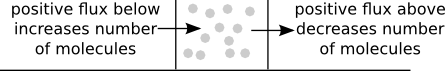
   Let's think about how the number of molecules in an small region around $x$ could change, as illustrated in the above diagram. The number of molecules in that region will increase if there is a positive flux $J$ just below $x$ (since that flux represents molecules arriving from below) and the number of molecules in that region will decrease if there is a positive flux $J$ just above $x$ (since that flux represents molecules leaving to go to larger values of $x$). Whether the number of molecules around $x$ is increasing or decreasing depends on whether the flux below or above is larger.

   The number of molecules at time $t$ will be proportional to the concentration at the point, $c(x,t)$. We can capture how this concentration $c(x,t)$ changes based on the flux above and below it using a continuity equation of the form $$\pdiff{c}{t}(x,t) = - \pdiff{J}{x}(x,t).$$ The continuity equation captures the fact that the concentration only changes due to the movement of molecules determined by the flux $J$. Rather than derive this equation, your task is to make an argument why the form of the continuity equation makes sense.

   Include the following pieces in your argument.

   • What does the partial derivative $\pdiff{J}{x}(x,t)$ mean (in terms of how $J$ changes as one of the variables changes)?
   • One special case of the equation is when $\pdiff{J}{x}(x,t)=0$. Justify that it makes sense that $\pdiff{c}{t}(x,t)$ would be zero in this case. Some steps could include:
     • If $\pdiff{J}{x}=0$, what does that mean about the flux $J(x,t)$? (In particular, what does that imply about the flux just above and just below a point $x$, as in the above illustration.)
     • If $\pdiff{c}{t} = 0$, what does that mean about the concentration $c(x,t)$?
     • If the flux $J(x,t)$ is of that form, why should that imply that the concentration won't change?
   • Imagine that $\pdiff{J}{x}(x,t) > 0$ at some point $x$. What does that mean about the flux just above and just below that point? Why would that form of the flux imply that the concentration $c(x,t)$ at $x$ should decrease?
   • Imagine that $\pdiff{J}{x}(x,t) < 0$ at some point $x$. What does that mean about the flux just above and just below that point? Why would that form of the flux imply that the concentration $c(x,t)$ at $x$ should increase?
4. The continuity equation is a general equation that includes cases beyond diffusion, depending on the form for the flux $J(x,t)$. When we account for the manner in which the molecules diffuse, we will obtain a form of the flux $J(x,t)$ that will turn the continuity equation into the diffusion equation.

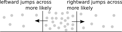
   The above diagram illustrates an important feature of diffusion. Since the jumps of each molecule occur randomly either left or right, whether the flux across a point $x$ is more rightward or leftward depends only on whether there are more molecules immediately to the right or the left. The rightward arrow indicates where the flux would be positive as the higher concentration of molecules to the left will lead to more rightward jumps across that point. The leftward arrow indicates the reverse situation, where the negative flux of more leftward jumps is caused by the higher concentration to the right.

   It turns out that, if the molecules are diffusing with diffusion coefficient $D$, the actual form of the flux will depend on the derivative of $c(x,t)$ with respect to $x$ according to the equation $$J(x,t) = -D\pdiff{c}{x}(x,t).$$ Make an argument why this form of the flux makes sense.

   Include the following pieces in your argument.

   • One special case is when $\pdiff{c}{x}=0$. Justify that it makes sense that the flux $J(x,t)$ should be zero in this case. (Recall that $J(x,t)$ is the net rate of molecules jumping rightward across $x$. When $J(x,t)=0$, does that mean molecules are not jumping rightward? Rather, what does it mean about the rightward and leftward jumps? Why should that be true when $\pdiff{c}{x}=0$?)
   • When $\pdiff{c}{x}(x,t) > 0$, what does this mean about the concentration $c(x,t)$. In that case, in which direction would you expect the net flux to be? Does this agree with the equation for $J(x,t)$?
   • When $\pdiff{c}{x}(x,t)< 0$, what does this mean about the concentration $c(x,t)$. In that case, in which direction would you expect the net flux to be? Does this agree with the equation for $J(x,t)$?

   The conclusion of this argument should be that the equation for $J(x,t)$ captures the fact that, with diffusion, molecules tend move from regions of higher concentration to regions of lower concentration.

5. Show how, combining the continuity equation with the equation for $J(x,t)$, one obtains the diffusion equation $$\pdiff{c}{t} = D \pdiffn{c}{x}{2}.$$ When combined with the boundary conditions you determined above, along with an initial condition $c(x,0) = f(x)$ for some initial condition $f(x)$, the diffusion equation determines the dynamics of the concentration $c(x,t)$.

The diffusion equation is a partial differential equation. Solving this equation to determine the dynamics of $c(x,t)$ is well beyond the scope of this project. Instead, we will look at the steady state solution $c(x)$, i.e., the equilibrium solution where $\pdiff{c}{t}=0$.

1. If the concentration is at steady state, then $\pdiff{c}{t}=0$, which means that $c(x,t)$ does not depend on $t$. We can write it as $c(x)$. Rewrite the diffusion equation in the steady state. Since $x$ is now the only variable, you can rewrite the partial derivatives with respect to $x$ as ordinary derivatives. We have transformed the partial differential equation to a much simpler ordinary differential equation.
2. Does the steady state equation actually depend on the diffusion coefficient $D$? If you can, cancel out the diffusion coefficient to rewrite the steady state equation in a simpler form.
3. If the steady state equation doesn't depend on $D$, then the steady state concentration $c(x)$ doesn't depend on $D$. Does that mean that diffusion coefficient does not influence the dynamics of the full partial differential equation? How might the diffusion coefficient influence how the concentration $c(x,t)$ approaches the steady state $c(x)$?
4. The steady state equation should involve a second derivative $\diffn{c}{x}{2}$. Solve this differential equation to determine what form $c(x)$ must be. It will involve two arbitrary constants, which you can call $C_1$ and $C_2$.

   You can determine the form of $c(x)$ by interpreting what the differential equation implies about the shape of the graph of $c$. Or, if you prefer, you can follow the following steps to determine the solution $c(x)$. In either case, be sure to plug in your form for $c(x)$ into the differential equation to verify that it solves the differential equation.

   Possible steps to determine the solution $c(x)$.

   1. The first step toward solving the equation is solving for the first derivative $\diff{c}{x}$. Let $g(x)=\diff{c}{x}(x)$ be this first derivative, which means that the second derivative $\diffn{c}{x}{2}$ is just the first derivative of $g(x)$: $\diffn{c}{x}{2} = \diff{g}{x}$. Rewrite the steady state diffusion equation as an equation for $g(x)$.
   2. The equation for the derivative $\diff{g}{x}$ should be very simple. From this equation, what must be the form of $g(x)$? You can't yet determine exactly what $g(x)$ is; it will involve an unknown constant. Call this constant $C_1$. Write a solution for $g(x)$ in terms of the constant $C_1$.
   3. Next, recall that $\diff{c}{x}(x)=g(x)$. Since you have determined $g(x)$, you now have an equation for $\diff{c}{x}$. If the slope of $c(x)$ is this value of $g(x)$, what must be the form of $c(x)$? It will involve yet another arbitrary constant, which you can call $C_2$.
5. Using the two boundary conditions, determine the values of the constants $C_1$ and $C_2$. Give the resulting steady state solution $c(x)$. This steady state solution will depend on two parameters: the concentration $c_0$ outside the cell and the length $L$.

   Sketch the graph of $c(x)$ over the interval $x \in (0,L)$.

6. Calculate the total number of molecules $N$ in the interval $x \in (0,L)$, which is the integral of the concentration over that interval: $N=\int_0^L c(x)dx$.
7. Since at state steady, the flux is $J(x) = -D \diff{c}{x}(x)$, calculate the flux of molecules into the cell, i.e., calculate $J(0)$.
8. So far, we've determined that, at steady state, molecules are entering the cell at a rate of $J(0)$. Since the system is at steady state, molecules must be removed at $x=L$ at the exact same rate $J(0)$ (otherwise the number of molecules in the interval $(0,L)$ would be changing, contradicting the fact that we are at steady state).

   We could equivalently say that a molecule enters the cell on average every $\tau = 1/J(0)$ seconds. In other words, on average, every $\tau$ seconds, one molecule is entering the cell at $x=0$ and one molecule is being removed at $x=L$.

   We want to know, on average, how long it takes a single molecule to diffuse from $x=0$ to $x=L$. Since there are $N$ molecules in the interval $(0,L)$ and a molecule is entering and being removed every $\tau$ seconds, it must be true that each molecule is taking, on average, $N\tau$ seconds to diffuse to $X=L$.

   We can justify that this average time must be $N\tau$ with the following argument.

   • To start with a trivial case where the argument is simple, let's imagine what would be true if $N$ were 1, i.e., that there were only one molecule in the interval $(0,L)$. Since we know that every $\tau$ seconds, one molecule enters at $x=0$ and another molecule is removed at $x=L$, we could conclude that the one molecule would have to race from $x=0$ to $x=L$ in those $\tau$ seconds; otherwise, there wouldn't be a molecule that could be removed after $\tau$ seconds.
   • If, on the other hand, there happened to be two molecules, each molecule could move at half the speed, making the trip from $x=0$ to $x=L$ in $2\tau$ seconds. Since a molecule would enter and be removed every $\tau$ seconds, this scenario is consistent with the requirements.
   • In reality, though, the number of molecules $N$ is much larger, meaning each molecule has a much longer time to make the trip from $x=0$ to $x=L$. Each molecule, on average, must take $N\tau$ seconds to make the trip.

   In summary, if there are $N$ molecules in the interval $(0,L)$ and molecules are entering the cell at $x=0$ at a rate of $J(0)$ while being removed at the same rate at $x=L$, then for everything to work out consistently, the average time for a molecule to diffuse from $x=0$ to $x=L$ must be $N/J(0)$ seconds, which is the same as $N\tau$ seconds where $\tau=1/J(0)$.

   Calculate the average time for a molecule to diffuse from $x=0$ to $x=L$ in terms of the length $L$ and the diffusion coefficient $D$. It turns out that the external concentration $c_0$ doesn't matter, and it should drop out of the equation for the average transport time.