An introduction to the directional derivative and the gradient
The directional derivative
Let the function $f(x,y)$ be the height of a mountain range at each point $\vc{x} = (x,y)$. If you stand at some point $\vc{x}=\vc{a}$, the slope of the ground in front of you will depend on the direction you are facing. It might slope steeply up in one direction, be relatively flat in another direction, and slope steeply down in yet another direction.
The partial derivatives of $f$ will give the slope $\pdiff{f}{x}$ in the positive $x$ direction and the slope $\pdiff{f}{y}$ in the positive $y$ direction. We can generalize the partial derivatives to calculate the slope in any direction. The result is called the directional derivative.
The first step in taking a directional derivative, is to specify the direction. One way to specify a direction is with a vector $\vc{u}=(u_1,u_2)$ that points in the direction in which we want to compute the slope. For simplicity, we will insist that $\vc{u}$ is a unit vector. We write the directional derivative of $f$ in the direction $\vc{u}$ at the point $\vc{a}$ as $D_{\vc{u}}f(\vc{a})$. We could define it with a limit definition just as an ordinary derivative or a partial derivative \begin{align*} D_{\vc{u}}f(\vc{a}) = \lim_{h \to 0} \frac{f(\vc{a}+h\vc{u}) - f(\vc{a})}{h}. \end{align*} However, it turns out that for differentiable $f(x,y)$, we won't need to worry about that definition.
The concept of the directional derivative is simple; $D_{\vc{u}}f(\vc{a})$ is the slope of $f(x,y)$ when standing at the point $\vc{a}$ and facing the direction given by $\vc{u}$. If $x$ and $y$ were given in meters, then $D_{\vc{u}}\vc{f}(\vc{a})$ would be the change in height per meter as you moved in the direction given by $\vc{u}$ when you are at the point $\vc{a}$.
Note that $D_{\vc{u}}f(\vc{a})$ is a number, not a matrix. In fact, the directional derivative is the same as a partial derivative if $\vc{u}$ points in the positive $x$ or positive $y$ direction. For example, if $\vc{u}=(1,0)$, then $\displaystyle D_{\vc{u}}f(\vc{a}) = \pdiff{f}{x}(\vc{a})$. Similarly if $\vc{u}=(0,1)$, then $\displaystyle D_{\vc{u}}f(\vc{a}) = \pdiff{f}{y}(\vc{a})$.
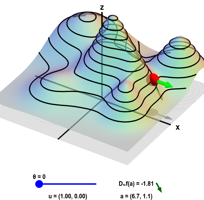
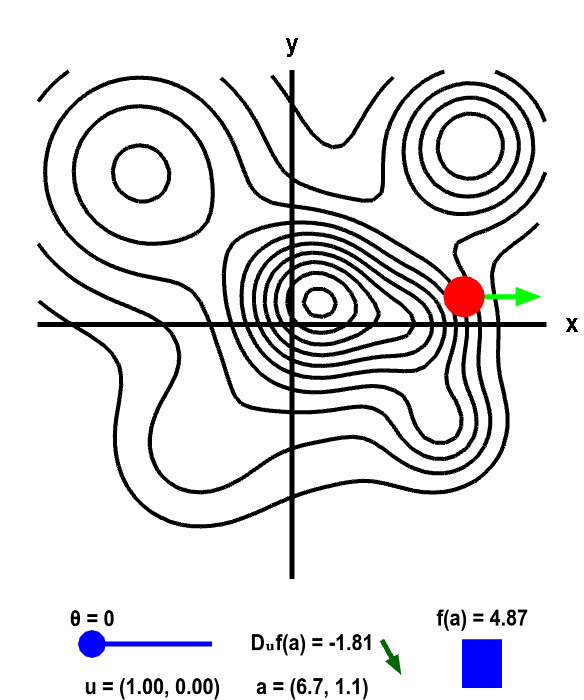
In the following applet, the height $f(x,y)$ of a mountain range is shown both as a surface plot (left) as a level curve plot (right). The interpretation of the two-dimensional point $\vc{a}$ and two-dimensional direction vector $\vc{u}$ defining the directional derivative $D_{\vc{u}}f(\vc{a})$ may be clearer in the two-dimensional level curve plot, so we focus on that panel first. You can recognize steep mountain peaks in the level curve plot by the closely spaced circular level curves. In this applet, you can move the point $\vc{a}$ around, change the direction $\vc{u}$ and observe how the directional derivative $D_{\vc{u}}f(\vc{a})$ changes. If you set $\vc{u}$ to point straight east ($\theta=0$ in the applet), then $\vc{u}$ points in the positive $x$ direction ($\vc{u}=(1,0)$) so that $\displaystyle D_{\vc{u}}f(\vc{a}) = \pdiff{f}{x}(\vc{a})$. Similarly, when $\vc{u}$ points straight north ($\theta=\pi/2$), then $\vc{u}$ points in the positive $y$ direction ($\vc{u}=(0,1)$) so that $\displaystyle D_{\vc{u}}f(\vc{a}) = \pdiff{f}{y}(\vc{a})$.
Applet loading
Applet loading
Directional derivative on a mountain. The height of a mountain range described by a function $f(x,y)$ is shown as surface plot in three-dimensions (left) and a two-dimensional level curve plot (right). In each panel, a red point can be moved by the mouse to change where the directional derivative is evaluated. The directional derivative is computed in the direction of the two-dimensional vector $\vc{u}$. This direction is illustrated by the light green vectors, and the value of the direction $\vc{u}$ is shown in the lower left of each panel. The direction of $\vc{u}$ is determined by the angle $\theta$ it makes with straight east (positive $x$ direction). The angle $\theta$, and hence $\vc{u}$, can be changed using the slider. The two-dimensional point $\vc{a}$ where the directional derivative is computed is illustrated by the shadow of the red point on the $xy$-plane below the surface plot and by the red point itself on the level curve plot. The value of the directional derivative $D_{\vc{u}}f(\vc{a})$ is shown at the bottom of the panel, along with the value of $\vc{a}$ itself. The value of $D_{\vc{u}}f(\vc{a})$ is the slope of the dark green vector to its right. This dark green vector is also shown emanating from the red point on the surface plot, where it is tangent to the surface, indicating that this slope is indeed the slope of the surface in the direction given by $\vc{u}$. The height of the surface $f(\vc{a})$ is illustrated by the bar in the lower right of the second panel.
If you make $\vc{u}$ point in a direction parallel to the level curve, what happens to $D_{\vc{u}} f(\vc{a})$? (Since the height is constant along a level curve, you should be able to infer what the slope in that direction should be.) Starting in any direction $\vc{u}$, what happens to $D_{\vc{u}}f(\vc{a})$ when you turn $\vc{u}$ to point in the opposite direction (i.e., add or subtract $\pi$ from $\theta$)?
In the surface plot, the steepness of the mountain may be easier to see. However, this view is a little misleading because it may lead you to think that the point $\vc{a}$ and the direction vector $\vc{a}$ are in three dimensions when they are really in two dimensions. In the surface plot, the red dot now floats in three dimensions on the surface of the mountain. Hence, the red dot in the surface plot is not $\vc{a}$; instead $\vc{a}$ is represented by the shadow of $\vc{a}$ on the $xy$-plane. Second, the light green vector representing $\vc{u}$ is floating on the surface. A better representation of the two-dimensional direction vector $\vc{u}$ is the shadow of the light green vector on the $xy$-plane.
The surface plot, though, is useful for recognizing that the directional derivative $D_{\vc{u}}f(\vc{a})$ is the slope of the surface. The dark green vector points up or down the mountain in the direction given by $\vc{u}$. The slope of this vector (which is the same thing as the slope of the surface) is the directional derivative. This vector (rotated to point toward the right) is displayed next to the value of $D_{\vc{u}}f(\vc{a})$ to further emphasize this point.
The gradient
In most cases, there is always one direction $\vc{u}$ where the directional derivative $D_{\vc{u}}f(\vc{a})$ is the largest. This is the “uphill” direction. (In some cases, such as when you are at the top of a mountain peak or at the lowest point in a valley, this might not be true.) Let's call this direction of maximal slope $\vc{m}$. Both the direction $\vc{m}$ and the maximal directional derivative $D_{\vc{m}}f(\vc{a})$ are captured by something called the gradient of $f$ and denoted by $\nabla f(\vc{a})$. The gradient is a vector that points in the direction of $\vc{m}$ and whose magnitude is $D_{\vc{m}}f(\vc{a})$. In math, we can write this as $\displaystyle \frac{\nabla f(\vc{a})}{\| \nabla f(\vc{a})\|} = \vc{m}$ and $\| \nabla f(\vc{a})\| = D_{\vc{m}}f(\vc{a})$.
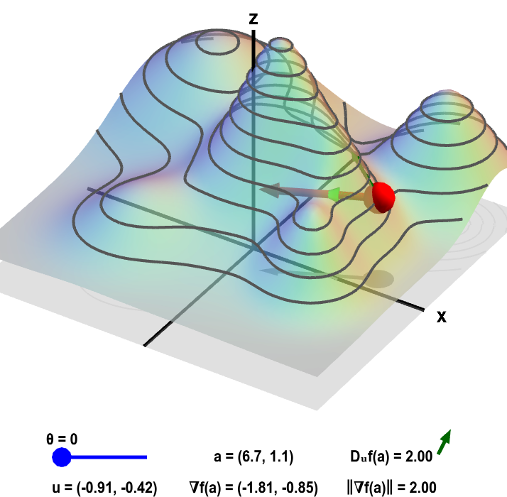
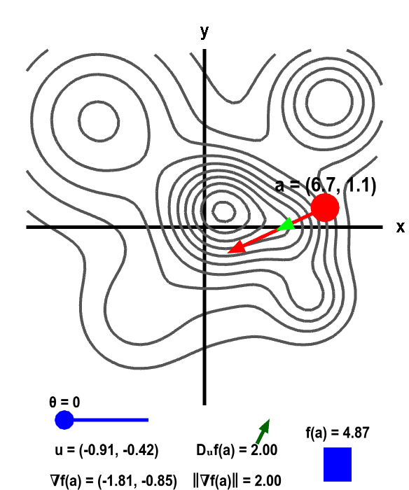
The below applet illustrates the gradient, as well as its relationship to the directional derivative. The definition of $\theta$ is different from that of the above applets. Here $\theta$ is the angle between the gradient and vector $\vc{u}$. When $\theta=0$, $\vc{u}$ points in the same direction as the gradient (and is hard to see in the applet).
Applet loading
Applet loading
Gradient and directional derivative on a mountain. The height of a mountain range described by a function $f(x,y)$ is shown as surface plot in three-dimensions (left) and a two-dimensional level curve plot (right). In each panel, a red point can be moved by the mouse to change the location $\vc{a}$ where the gradient $\nabla f(\vc{a})$ is calculated. Since $f$ is a function of two variables, the point $\vc{a}$ and the gradient are two-dimensional. The two-dimensional point $\vc{a}$ is illustrated by the shadow of the red point on the $xy$-plane below the surface plot and by the red point itself on the level curve plot. The two dimensional gradient vector $\nabla f(\vc{a})$ is illustrated by the red vector emanating from the red point as well as by its shadow below the surface plot.
The light green two-dimensional vector $\vc{u}$ points at an angle $\theta$ (changeable via the slider) from the gradient. (It is also represented by its shadow below the surface plot.) The value of the directional derivative $D_{\vc{u}}f(\vc{a})$ is the slope of the dark green vector tangent to the surface, which is reproduced next to the value of $D_{\vc{u}}f(\vc{a})$ shown at the bottom of each panel. The value of the directional derivative is compared to the magnitude of the gradient $\| \nabla f(\vc{a})\|$. The height of the surface $f(\vc{a})$ is also illustrated by the bar in the lower right of the second panel.
Notice how the red gradient vector always points up the mountains (in fact, the gradient is always perpendicular to the level curves). When the level curves are close together, the gradient is large. What happens to the gradient at the tops of the mountains?
Note that when $\theta=0$ (or $\theta = 2\pi$), the directional derivative $D_{\vc{u}}f(\vc{a})$ and the magnitude of the gradient $\|\nabla f (\vc{a})\|$ are identical, i.e., $D_{\vc{u}}f(\vc{a}) = \| \nabla f(\vc{a})\|$. When $\theta=\pi$, then $\vc{u}$ points in the opposite direction of the gradient, and $D_{\vc{u}}f(\vc{a}) = - \| \nabla f(\vc{a})\|$. For what values of $\theta$ is $D_{\vc{u}}f(\vc{a}) = 0$?
By moving $\vc{a}$ (the dark red point) around and changing $\theta$, I hope you can convince yourself that, for a fixed $\vc{a}$, the maximal value of $D_{\vc{u}}f(\vc{a})$ occurs when $\vc{u}$ and $\nabla f (\vc{a})$ point in the same direction (i.e., when $\theta=0$ or $\theta=2\pi$), and the minimum value occurs when $\vc{u}$ and $\nabla f (\vc{a})$ point in opposite directions (i.e., when $\theta=\pi$). Hence $D_{\vc{u}}f(\vc{a})$ always lies between $-\| \nabla f(\vc{a})\|$ and $\| \nabla f(\vc{a})\|$. It turns out that the relationship between the gradient and the directional derivative can be summarized by the equation \begin{align*} D_{\vc{u}}f(\vc{a}) &= \nabla f(\vc{a}) \cdot \vc{u}\\ &= \|\nabla f(\vc{a})\|\, \| \vc{u}\| \cos\theta\\ &= \| \nabla f(\vc{a})\| \cos\theta \end{align*} where $\theta$ is the angle between $\vc{u}$ and the gradient. (Recall that $\vc{u}$ is a unit vector, meaning that $\| \vc{u}\|=1$.)
But what exactly is the gradient?
This page was designed to give you an intuitive feel for what the directional directive and gradient are. But, we've failed to mention what exactly is the gradient. The above formula for the directional derivative is nice, but it's not very useful if you don't know how to calculate $\nabla f$. Fortunately, the end result is fairly simple, as the gradient is just a reformulation of the matrix of partial derivatives. You can check out a simple derivation of the gradient to see why this is true.
Once you know how to calculate the gradient, you can follow these examples.
Thread navigation
Multivariable calculus
- Previous: Multivariable chain rule examples
- Next: Derivation of the directional derivative and the gradient
Math 2374
- Previous: Orienting curves
- Next: The gradient vector
Similar pages
- Derivation of the directional derivative and the gradient
- Subtleties of differentiability in higher dimensions
- The derivative matrix
- Directional derivative and gradient examples
- The multidimensional differentiability theorem
- Non-differentiable functions must have discontinuous partial derivatives
- A differentiable function with discontinuous partial derivatives
- Introduction to partial derivatives
- Partial derivative examples
- Partial derivative by limit definition
- More similar pages