Introduction to differentiability in higher dimensions

Review of differentiability in one-variable calculus

You learned in one-variable calculus that a function $f: \R \to \R$ (confused?) may or may not be differentiable. In fact, a function may be differentiable at some places but not in others.

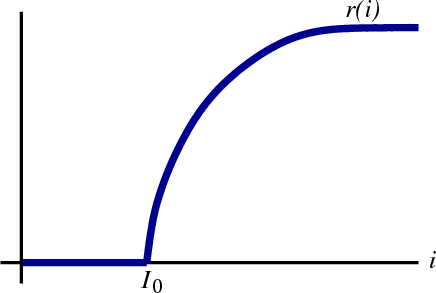
Consider the function $r(i)$ that gives the output rate $r$ of a neuron as a function of its input $i$. A neuron communicates to other neurons by sending output pulses (or “spikes”) to other neurons. For simplicity, we only keep track of the rate $r(i)$ of these spikes. Since a negative rate isn't meaningful, we know that $r(i) \ge 0$.

For this idealized neuron model, the neuron is completely silent when it has very little input, i.e., when the input $i$ is small then the rate $r(i)=0$. Only when the input exceeds some threshold $I_0$ does the neuron begin emitting output spikes. The output rate increases as $i$ increases, as illustrated in this graph of $r(i)$. (The curve levels off for high values of $i$ because there is a limit on how fast the neuron can emit output spikes. For example, the limit might be 200 spikes per second.)

The function is differentiable everywhere except at the point where $i = I_0$. By differentiable, we mean that we can fit the graph of $r(i)$ with a (non-vertical) tangent line. Given any level of input, say $i=a$, we can find a line that closely approximates $r(i)$ around $a$, as long as $a \ne I_0$.

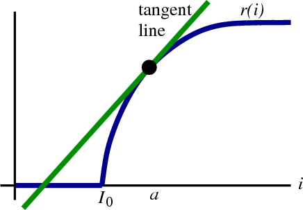
The function $r(i)$ is not differentiable at $i = I_0$ because there is no tangent line at $i=I_0$. The graph of $r$ has a kink there, so no matter what line we chose, it will fail to match the graph on either the left or the right side of $I_0$.

An equation for a line through the point $(a,r(a))$ (shown as the black point in the figure) is \begin{align*} L(i) = r(a) + m(i-a), \end{align*} where $m$ is the slope of the line. We can think of the fact that “$r(i)$ is differentiable at $i=a$” as meaning that $r(i)$ is nearly linear for $i$ near $a$. We can find a particular value of the slope $m$ so that the line $L(i)$ is a very good approximation for $r(i)$ when $i$ is close to $a$. For this particular value of $m$, the line $L(i)$ is called the the linear approximation to $r(i)$ around $a$. This line is, of course, the tangent line to $r$.

The particular slope where $L(i)$ becomes the tangent line, or linear approximation, is the derivative $m=r'(a)$. You've learned other definitions of the derivative of a function, but you could just as well define it as the slope of this linear approximation. This is, in effect, how we will define the derivative in higher dimensions.

Differentiability in two dimensions

The purpose that long-winded review of one-variable differentiability was to recast the derivative into the language we will use for multivariable differentiability.

To illustrate, let's modify our neuron example. In turns out many neurons have “receptors” built right into them that respond to nicotine. For these neurons, the presence of nicotine alters their behavior. (Needless to say, many in the medical community are interested in the nicotine receptors as nicotine is a common drug of addiction.) We can model the effects of nicotine by defining a new function $r : \R^2 \to \R$ that gives the neural response as a function of both input $i$ and nicotine level $s$. (The choice of the letter $s$ comes from “smoke.”)

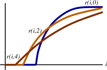
Let's pretend that the effect of nicotine is to shift the threshold $I_0$ to smaller values and flatten out a neuron's response to input. We write the response of a neuron to input $i$ and nicotine $s$ as $r(i,s)$. If we look at the case when $s=0$, we have the original curve $r(i,0)$ of neural output rate to input. If we add nicotine so some level, say $s=2$ (in some arbitrary units), then the curve becomes $r(i,2)$, a shifted and flattened version of the original curve. Increasing nicotine further to $s=4$ gives the further shifted and flattened curve $r(i,4)$.

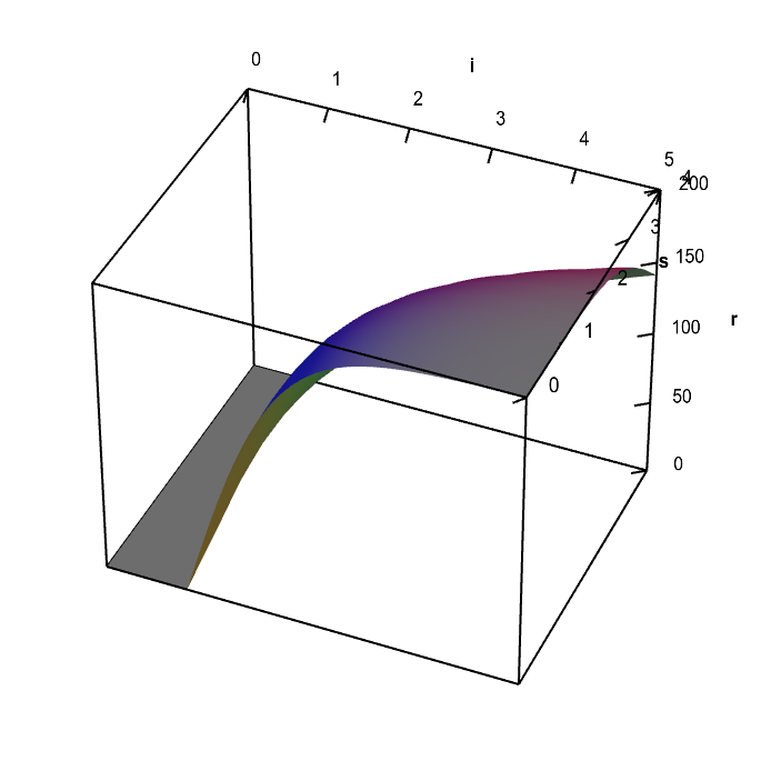
To get a complete picture, we can plot the full function $r(i,s)$. Here is an applet showing $r(i,s)$, which you can rotate to view better.

Applet: Neuron firing rate in response to input and nicotine levels

Applet loading

Neuron firing rate in response to input and nicotine levels. A fictitious representation of the firing rate $r(i,s)$ of a neuron in response to an input $i$ and nicotine level $s$. The firing rate increases with input $i$, but it increases more slowly as $s$ increases. The firing rate is zero below a threshold input that decreases with $s$. This leads to a fold in the surface that describes the function $r(i,s)$.

More information about applet.

One of the first things you may notice is that the surface $r(i,s)$ is smooth except for a fold or crease along a line. This fold is compoosed of those points where, for a given nicotine level $s$, $r(i,s)$ suddenly becomes nonzero as you increase the input $i$. The fold is analogous to the kink at $I_0$ that we saw in the original curve, above.

We want to define a notion of differentiability for our multivariable function $r(i,s)$. As in the one-variable case, the function $r(i,s)$ may be differentiable at some points and not at others. Our definition of differentiability should distinguish the fold in the surface from the smooth parts of the surface. To be consistent with the one-variable case, the function $r(i,s)$ should fail to be differentiable along the fold.

Given some point $\vc{a}=(a_1,a_2)$, the function $r(i,s)$ is differentiable at the point where $(i,s) = \vc{a}$ if it has a (non-vertical) tangent plane at $\vc{a}$. The definition of a tangent plane is analogous to the definition of a tangent line. At points $(i,s)$ near $\vc{a}$, the function $r(i,s)$ is nearly identical to the tangent plane.

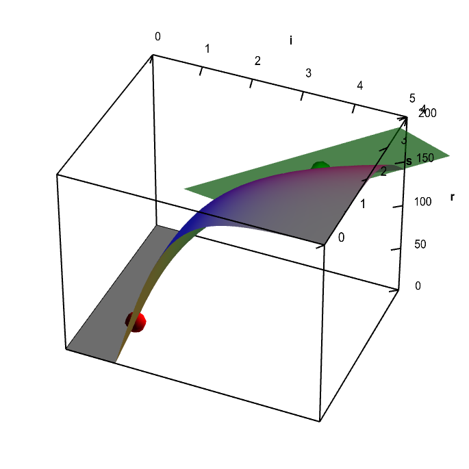
For example, the below graph shows that $r(i,s)$ is differentiable at the point $(i,s)=(3,3)$ (shown by the green dot), as there is a tangent plane at that point. On the other hand, if we tried to fit a plane at a point where the surface folds (e.g., the point shown by the red dot), we would never succeed. The plane will fail to match the graph on one side of the fold or the other. Hence the function $r(i,s)$ is not differentiable at any point along the fold.

Applet: Neuron firing rate function with tangent plane

Applet loading

Neuron firing rate function with tangent plane. A fictitious representation of the firing rate $r(i,s)$ of a neuron in response to an input $i$ and nicotine level $s$. The graph of the function has a tangent plane at the location of the green point, so the function is differentiable there. By rotating the graph, you can see how the tangent plane touches the surface at the that point. You can move the green point anywhere on the surface; as long as it is not along the fold of the graph (where the red point in constrained to be), you can see the tangent plane showing that the function is differentiable. There is no tangent plane to the graph at any point along the fold of the graph (you can move the red point to any point along this fold). The function $r(i,s)$ is not differentiable at any point along the fold. As further evidence of this non-differentiability, the tangent plane jumps to a different angle when you move the green point across the fold.

More information about applet.

An equation for a plane through the point $(a_1,a_2,r(a_1,a_2))$ (such as the green point in the applet) is given by \begin{align*} L(i,s) = r(a_1,a_2) + m(i-a_1) + n(s-a_2). \end{align*} In this case, we have two slopes: the slope $m$ in the direction where $i$ increases, and the slope $n$ in the direction where $s$ increases. If $r(i,s)$ is differentiable at $(a_1,a_2)$, that means $r$ is nearly linear for $(i,s)$ near $(a_1,a_2)$. Hence, we can find slopes $m$ and $n$ so that $f(i,s)$ is a really good approximation for $r(i,s)$ for $(i,s)$ close to $(a_1,a_2)$. For these particular values of $m$ and $n$, $L(i,s)$ is called the linear approximation to $r(i,s)$, i.e., $L(i,s)$ is the tangent plane.

What are these special values of $m$ and $n$? They are the slopes of the graph of $r(i,s)$ in the $i$ and $s$ direction, which are the partial derivatives of $r$ at $\vc{a}=(a_1,a_2)$: \begin{align*} m = \pdiff{r}{i}(a_1,a_2)\\ n = \pdiff{r}{s}(a_1,a_2). \end{align*}

In this way, the two-variable differentiability is analogous to the one-variable differentiability, with differentiability meaning the existence of the linear approximation. The linear approximation is just a bit more complicated: the tangent line with one slope is replaced by the tangent plane with two slopes. In the one-variable case, the one slope was the derivative. In the two-variable case, we group the two slopes together into the matrix of partial derivatives: \begin{align*} Dr(a_1,a_2) = \left[\pdiff{r}{i}(a_1,a_2) \,\, \,\, \pdiff{r}{s}(a_1,a_2)\right]. \end{align*} If the tangent plane exists at $\vc{a}=(a_1,a_2)$, we can think of the row matrix $Dr(\vc{a})$ as being the derivative of $r$ at the point $\vc{a}$.

In summary, if the function $r(i,s)$ has a tangent plane at the point $(i,s)=\vc{a}$, then it is differentiable at $\vc{a}$. The slopes of the tangent plane are the partial derivatives of $r$. The matrix of partial derivatives $Dr(\vc{a})$ is the derivative of the function $r(i,s)$ at the point $\vc{a}$. Similar to the one-variable case, the tangent plane $L(i,s)$ is called the linear approximation to $r(i,s)$. The fact that $r(i,s)$ is differentiable means that it is close to its linear approximation around $(i,s)=\vc{a}$.

We've just scratched the surface

In such a short introduction to differentiability, we've had to hide a lot of the important details under the rug. You may have noticed we played a little loose with the language in describing the differentiability condition as having a linear approximation, as we used phrases like a “really good” approximation to the function.

Once you feel comfortable with the basic idea of differentiability presented in this page, then we encourage you to take the next step to toward understanding what differentiability really means. One suggestion is to check out the actual definition of differentiability to learn what we meant when we said the linear approximation must be “really good” approximation to the function. (If this is your first time reading about differentiability, you might want to first go out and get some fresh air before continuing on.)

Differentiability in higher dimensions is trickier than in one dimension because with two or more dimensions, a function can fail to be differentiable in more subtle ways than the simple fold we showed in the above example. In fact, the matrix of partial derivatives can exist at a point without the function being differentiable at that point. That's right, the existence of all partial derivatives is not enough to guarantee differentiability. To really understand differentiability, you need to grapple with some of these subtleties of differentiability in higher dimensions.

Want to see some examples of calculating the derivative in higher dimensions?