Bacteria growth model exercise answers
Here we give answers to some of the bacteria growth exercises.
Exercise 1
\begin{align*} {\rm{a.}} \hspace{2mm} B_3 & = 1.5^3 \times 4 \\ {\rm{c.}} \hspace{2mm} B_3 & = 1.05^3 \times 0.2\\ {\rm{e.}} \hspace{2mm} B_3 & = 1.4^3 \times 100 \end{align*}
Exercise 2
\begin{align*} {\rm{a.}} \hspace{2mm} B_t & = 4 \times 1.5^t\\ {\rm{c.}} \hspace{2mm} B_t & = 0.2 \times 1.05^t\\ {\rm{e.}} \hspace{2mm} B_t & = 100 \times 1.4^t \end{align*}
Exercise 4
(a) The change in population is summarized in the following table.
| $t$ | $B_t$ | $B_{t+1}-B_t$ |
|---|---|---|
| 0 | 1.99 | 0.69 |
| 1 | 2.68 | 0.95 |
| 2 | 3.63 | 1.26 |
| 3 | 4.89 | 1.74 |
| 4 | 6.63 | 2.30 |
| 5 | 8.93 | 3.17 |
| 6 | 12.10 |
Using the population change line fitting applet, the points could be fit by a line through the origin with slope $r=0.35$, as shown below.
Fitting a linear model to population change versus population size, answer to bacteria exercise 4a.
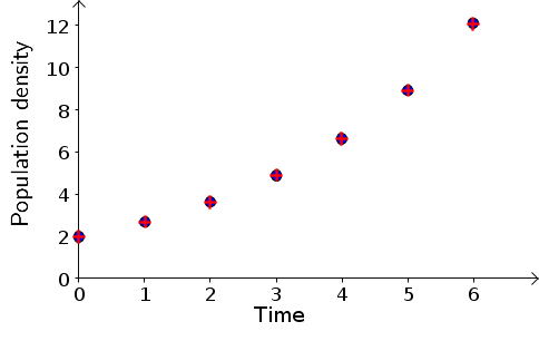
With $r=0.35$, the model values for the points are shown in the following table.
| $t$ | Data $B_t$ | Model $B_t$ |
|---|---|---|
| 0 | 1.99 | 1.99 |
| 1 | 2.68 | 2.69 |
| 2 | 3.63 | 3.63 |
| 3 | 4.89 | 4.90 |
| 4 | 6.63 | 6.61 |
| 5 | 8.93 | 8.92 |
| 6 | 12.10 | 12.05 |
The model points are very close to the data points, as shown in the following figure. Blue circles are data points; red cross are model points.
If you click the image, you can download the Geogebra source file that may help you use Geogebra to produce such an image.
(c) The change in population is summarized in the following table.
| $t$ | $B_t$ | th>$B_{t+1}-B_t$|
|---|---|---|
| 0 | 22.1 | 1.3 |
| 1 | 23.4 | 2.7 |
| 2 | 26.1 | 1.4 |
| 3 | 27.5 | 3.0 |
| 4 | 30.5 | 3.9 |
| 5 | 34.4 | 2.2 |
| 6 | 36.6 |
Using the population change line fitting applet, the points could be fit by a line through the origin with slope $r=0.08$, as shown below.
Fitting a linear model to population change versus population size, answer to bacteria exercise 4c.
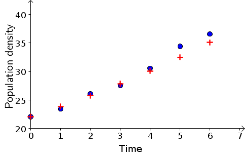
With $r=0.08$, the model values for the points are shown in the following table.
| $t$ | Data $B_t$ | Model $B_t$ |
|---|---|---|
| 0 | 22.1 | 22.1 |
| 1 | 23.4 | 23.87 |
| 2 | 26.1 | 25.78 |
| 3 | 27.5 | 27.84 |
| 4 | 30.5 | 30.07 |
| 5 | 34.4 | 32.47 |
| 6 | 36.6 | 35.07 |
The model points are somewhat close to the data points, as shown in the following figure. Blue circles are data points; red cross are model points.
Exercise 5
In a plot of $B_{t+1}-B_t$ versus $B_t$, the first four points fall close to a line. The slope of the line is approximately 0.7. An approximate model is \[ B_{t+1} - B_t = 0.7 B_t \]
The means that approximately 70 percent of the cells divide in each time interval, which is slightly more than we found for a pH of 6.25. A solution to the dynamical system is \[ B_t = B_0 \times 1.7^t = 0.028 \times 1.7^t. \]
The resulting values from the model are close to those of the data except, perhaps, for the last value.
Similar pages
- Developing an initial model to describe bacteria growth
- Bacteria growth model exercises
- Environmental carrying capacity
- Developing a logistic model to describe bacteria growth
- Harvest of natural populations
- Harvest of natural populations exercises
- Harvest of natural populations exercise answers
- The idea of a dynamical system
- An introduction to discrete dynamical systems
- Exponential growth and decay modeled by discrete dynamical systems
- More similar pages