The idea of a dynamical system
What is a dynamical system?
A dynamical system is all about the evolution of something over time. To create a dynamical system we simply need to decide (1) what is the “something” that will evolve over time and (2) what is the rule that specifies how that something evolves with time. In this way, a dynamical system is simply a model describing the temporal evolution of a system.
The state space
The first step in creating a dynamical system is to pin down what is the special “something” that we want to evolve with time. To do this, we need to come up with a set of variables that give a complete description of the system at any particular time.
By “complete description,” we don't necessarily mean that the variables will completely describe a real life system we may be trying to model. But, the variables must completely describe the state of the mathematical system. In a dynamical system, if we know the values of these variables at a particular time, we know everything about the state of the system at that time. To model some real life system, the modeler must clearly make a choice of what variables will form the complete description for the mathematical model.
The variables that completely describe the state of the dynamical system are called the state variables. The set of all the possible values of the state variables is the state space.
The state space can be discrete, consisting of isolated points, such as if the state variables could only take on integer values. It could be continuous, consisting of a smooth set of points, such as if the state variables could take on any real value. In the case where the state space is continuous and finite-dimensional, it is often called the phase space, and the number of state variables is the dimension of the dynamical system. The state space can also be infinite-dimensional.
The time evolution rule
The second step in creating a dynamical system is to specify the rule for the time evolution of the dynamical system. This rule must be defined to make the state variables be a complete description the state of the system in the following sense: the value of the state variables at a particular time must completely determine the evolution to all future states. If the time evolution depends on a variable not included in the state space, then the rule combined with the state space does not specify a dynamical system. One must either change the rule or augment the state space by the neccesary variables to form a dynamical system.
The time evolution rule could involve discrete or continuous time. If the time is discete, then the system evolves in time steps, and we usually let the time points be the integers $t=0,1,2,\ldots.$ We can write the state of the system at time $t$ as $x_t$. In many cases, the time evolution rule will be based on a function $f$ that takes as its input the state of the system at one time and gives as its output the state of the system at the next time. Therefore, starting at the initial conditions $x_0$ at time $t=0$, we can apply the function once to determine the state $x_1=f(x_0)$ at time $t=1$, apply the function a second time to get the state $x_2=f(x_1)$ at time $t=2$, and continue repeatedly applying the function to determine all future states. We end up with a sequence of states, the trajectory of the point $x_0$: $x_1, x_2, x_3, \ldots.$ In this way, the state at all times is determined both by the function $f$ and the initial state $x_0$. We refer to such as system as a discrete dynamical system.
In a continuous dynamical system, on the other hand, the state of the system evolves through continuous time. One can think of the state of the system as flowing smoothly through state space. As time evolves, the state $x(t)$ at time $t$ can be thought of as a point that moves through the state space. The evolution rule will specify how this point $x(t)$ moves by giving its velocity, such as through a function $v(t)=F(x(t))$, where $v(t)$ is the velocity of the point at time $t$. In this case, starting with an initial state $x(0)$ at time $t=0$, the trajectory of all future times $x(t)$ will be a curve through state space.
Examples of dynamical systems
To illustrate the idea of dynamical systems, we present examples of discrete and continuous dynamical systems.
Bacteria doubling example
The first dynamical system will model the growth of a bacteria population. Let the population size $b_t$ be the number of bacteria in the population at time $t$. If we allow the values of the $b_t$ to be non-negative integers, then the non-negative integers form the state space, and the state space is discrete.
The bacteria population grows because each baterium grows and the divides into two bacteria. For this example, we will assume that all the bacteria divide at the same time. Then, we can define one time step as the time for all the bacteria to divide into two. For this model, we ignore how much real time elapses between each division cycle, but define our time so that one unit of time is the time between divisions. In this way, we form a discrete dynamical system, and simply need a rule to determine the population size $b_t$ at the times $t=1,2,3, \ldots$ given the initial population size $b_0$ at time $t=0$.
Since every bacterium divides into two during each time step, the rule is particular simple. The population size doubles at each time step. For any time $t=n$, the population size at the next step $b_{n+1}$ will be two times the previous population size $b_n$, i.e., $b_{n+1}=f(b_n)=2b_n$.
The rule $b_{n+1}=2b_n$, coupled with the initial population size $b_0$ at time $t=0$, completely determines the population size at all future times $t$. Our dynamical system is well defined.
The bacteria doubling dynamical system is illustrated by the following applet, which shows a number of ways to represent the solution trajectory $b_1, b_2, b_3, \ldots.$ In this example, the dependence of the solution on the initial state $b_0$ is quite simple. The trajectory is just scaled by $b_0$.
Bacteria doubling. The evolution of this bacteria population follows a simple rule: the number of bacteria doubles every time step. Since the state of the system is determined by a single variable, the population size $b$, the state space is one-dimensional. The state space is represented by the blue vertical line at the left. The initial population size $b_0$ is a blue point and the population size $b_t$ at time $t$ is a red point on this state space. The time evolution of the dynamical system is also represented by the plot of population size $b_t$ versus $t$, where the lines connecting the points are not part of the graph but are there just to guide your eye. The population size $b_t$ is also illustrated in the right panel where each green dot represents one bacterium. You can change the time $t$ and the initial population size $b_0$ by moving the sliders in the gray box. Stop or start the animation by clicking the button that appears in the lower left corner of one of the panels.
In the above description of this example, we defined the state space to be the non-negative integers. The mathematical system will work the same way if we allow the population size to be any real number. Of course, it might be hard to interpret the meaning of fractional bacteria. But, as you learn how to analyze discrete dynamical systems, you will see how expanding the state space to include all real numbers will facilitate the mathematical analysis.
Undamped pendulum example
A second example dynamical system is a model of an undamped pendulum, that is, a pendulum that oscillates without any friction so that it will continue oscillating forever. Imagine that the pendulum consists of a rigid rod with a ball fastened at its end and that the pendulum is free to rotate around the pivot point.
We can specify the position of the pendulum by the angle $\theta$ that the rod makes with a line pointing straight down. The angle is zero when the pendulum points straight down, and $\theta = \pm\pi$ when the pendulum points straight up. We use the convention that $0 < \theta < \pi$ indicates that the pendulum is pointing toward the right and that $-\pi < \theta < 0$ indicates that the pendulum is pointing toward the left.
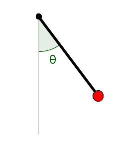
The angle $\theta$ completely specifies the position of the pendulum. So, our first thought might be that $\theta$ should completely determine the state of the dynamical system. However, we cannot use $\theta$ as the only state variable. If the above picture of the pendulum were a snapshot of a pendulum, we don't have enough information to know where the pendulum will move next.
We might think that the pendulum will start moving downward because we implicitly assume that the pendulum starts out being stationary. But, if I told you that when I took the snapshot of the pendulum, it was moving rapidly in a counterclockwise direction, the additional information of how the pendulum was moving at the time of the snapshot would change your prediction of where the pendulum will move next. If we know the pendulum pictured above has a counterclockwise velocity, we expect that the pendulum will continue to move upward.
In order to determine the future behavior of the pendulum, we need to know not only its position at the time of the snapshot, but also its velocity. Hence, the state space must include both those variables. It turns out that for this idealized pendulum, the angle $\theta$ and the angular velocity $\omega$ completely determine the state of the system. Both $\theta$ and $\omega$ will evolve over time, and their value at one time determines all their future values. The dynamical system is two-dimensional, and since $\theta$ and $\omega$ evolve continuously, it is a continuous dynamical system.
In the above bacteria dynamical system, we plotted the one-dimensional state space (or phase space) as a blue line. In the pendulum example, we can plot the two-dimensional state space (or phase space) as a plane, often called the phase plane. We can plot $\theta$ on the $x$-axis of the Cartesian plane and $\omega$ on the $y$-axis. In this representation, the current state of the system, $\theta(t)$ and $\omega(t)$, is a point $(\theta(t),\omega(t))$ on the phase plane, plotted as the red point on the left panel of the applet, below. The trajectory of the initial condition $(\theta(0),\omega(0))=(\theta_0,\omega_0)$ (the blue point labeled as $X_0$) is the green curve in the left panel.
To further help you visualize how $(\theta(t),\omega(t))$ flows through the state space, gray arrows indicating the velocity of $(\theta(t),\omega(t))$ are plotted throughout the phase plane. Not only do the arrows point out the direction of the flow, but their length indicates the speed of $(\theta(t),\omega(t))$.
Undamped pendulum. The dynamical system describing an undamped pendulum requires two state variables. The angle $\theta$ of the pendulum and the angular velocity $\omega$. These two variables completely describe the state of the pendulum. The state space (or phase space) $(\theta,\omega)$ is illustrated in the left panel. The space is periodic in $\theta$, and the range $-\pi \le \theta < \pi$ is shown. The initial angle and angular velocity, $\vc{X}_0 = (\theta_0,\omega_0)=(\theta(0),\omega(0))$, is set by dragging the blue point. The resulting evolution of the system is illustrated both by the green curve (the trajectory) and the moving red point, which indicates the state (i.e., angle and angular velocity) at time $t$: $(\theta(t),\omega(t))$. Gray arrows represent the speed and direction that the point $(\theta(t),\omega(t))$ moves through the state space. The right panel illustrates the evolution of just the angle $\theta(t)$ with respect to time $t$. The plot includes both the graph of $\theta$ versus $t$ in green and a moving red point, corresponding to the similar curve and point in the left panel. Above the graph are slider by which you can change the time $t$ and a graphical illustration of the pendulum with angle $\theta(t)$ and angular velocity $\omega(t)$. If the angular velocity $\omega$ is sufficiently large, the pendulum will swing around past an angle of $\pm\pi$. In this case, the variable $\theta(t)$ will wrap around from $\pi$ to $-\pi$ or vice versa. At those points, the green curves will contain extraneous lines crossing between $\theta=\pi$ and $\theta=-\pi$. Those lines should be ignored.
The state space isn't really a plane because the angle $\theta$ is $2\pi$-periodic. The left edge of the plane at $\theta=-\pi$ is really the same thing as the right edge of the plane at $\theta=\pi$, as both corresponding to the pendulum pointing straight up. You could imagine taking the phase plane plotted in the left panel and rolling it into a cylinder so that the lines $\theta=-\pi$ and $\theta=\pi$ match up. The cylinder would be a better representation of the phase space. The angular velocity $\omega$, however, is not periodic, as positive values indicate a counterclockwise rotation of the pendulum (shown as an inset in the right panel) and negative values indicate clockwise rotation.
The right panel of the above applet shows a plot of the pendulum angle $\theta$ versus time. Because the state space is two-dimensional, we can't easily plot the full system state $(\theta(t),\omega(t))$ versus time. Instead, we chose to just plot the angle. (We could have also included a separate plot of $\omega$ versus $t$.) Again, this plot should really be on a cylinder, as the top edge of the gray region is $\theta=\pi$ and the bottom edge is $\theta=-\pi$, which are really the same thing.
It may be slightly confusing that we have mentioned two different velocities. One velocity is the angular velocity $\omega(t)$, which tells us how fast the angle $\omega(t)$ is changing and in which direction. The second velocity is the velocity (speed and direction) of the point $(\theta(t),\omega(t))$ through state space, i.e., the velocity of the red point in the left panel, above. These two velocities are related, as the left and right movement of the red point is due to changes in $\theta(t)$. In fact, the velocity of this left and right movement is exactly given by the angular velocity. The up and down movement of the red point is given by changes in the angular velocity $\omega(t)$, or the acceleration of the pendulum. How $\omega(t)$ changes with time depends on a little physics, and a discussion of this mechanism is outside the scope of this introductory page.
Thread navigation
Elementary dynamical systems
Math 1241, Fall 2020
- Previous: Gateway exam
- Next: Introduction to Dynamical Systems
Math 201, Spring 22
Similar pages
- An introduction to discrete dynamical systems
- Developing an initial model to describe bacteria growth
- Bacteria growth model exercises
- Bacteria growth model exercise answers
- Exponential growth and decay modeled by discrete dynamical systems
- Discrete exponential growth and decay exercises
- Discrete exponential growth and decay exercise answers
- Doubling time and half-life of exponential growth and decay
- Constructing a mathematical model for penicillin clearance
- Penicillin clearance model exercises
- More similar pages