Developing an initial model to describe bacteria growth
Why bacteria?
One important dynamical process in biology is the growth of organisms and populations of organisms. In some species, individuals grow larger over time. But in all species, reproduction is imperative for survival. An important mark of a successful species is growth in its population size, meaning the number of individuals in the population.
The population growth of bacteria is relatively simple, at least under carefully controlled environments in the laboratory. For example, bacterial populations increase rapidly when grown at low bacterial densities in abundant nutrient. The population increase is due to binary fission, where single cells divide asexually into two cells, subsequently the two cells divide to form four cells, and so on. The time required for a cell to mature and divide is approximately the same for any two cells.
For this reason, bacteria population growth can serve as a basis for a simple discrete dynamical system model that introduces some key components of modeling dynamical processes. In developing a discrete dynamical system model for bacteria growth, we illustrate some of the steps in formulating a model and analyzing its properties, with the goal of using the model to deepen our insight into the underlying physical or biological process.
Developing a model from experimental data
Developing a bacteria growth model from experimental data.
Vibrio natriegens, or V. natriegens for short, is a marine bacterium commonly found in the mud around estuaries. One can manipulate the growth rate of V. natriegens in a laboratory by using simple manipulations of the experimental conditions. Our goal will be to build discrete dynamical system models describing its population growth under a few experimental conditions.
Bacterial growth data from a V. natriegens experiment are shown in the following table. The population was grown in a commonly used nutrient growth medium, but the pH of the medium was adjusted to be pH 6.25.1
| Time (min) | Population Density |
|---|---|
| 0 | 0.022 |
| 16 | 0.036 |
| 32 | 0.060 |
| 48 | 0.101 |
| 64 | 0.169 |
| 80 | 0.266 |
Visualizing population density versus time
The bacteria population size was recorded every 16 minutes, giving us precisely the snapshots we described in the discrete dynamical system introduction. We'll let $t$ denote time rescaled so that the time between snapshots is one unit of time. Then, the above snapshots occurred at times $t=0,1,2,3,4,5$. Time $t=3$, for example, indicates the actual time of $3 \times 16 = 48$ minutes.
The data consists of measurements of bacterial population density at each time point. In our discrete dynamical system model, this population density will be the single state variable in our state space, and we'll denote the bacterial density by $B$. Then $B_t$ is the snapshot of bacterial density at time point $t$. With this notation, we can write the data from the above table as $B_0 = 0.022$, $B_1 = 0.036$, $B_2 = 0.060$, etc.
With the state space and set of times determined, the remaining step in developing the dynamical system model is to determine the time evolution rule. This step, of course, is the most difficult part, as it must capture the dynamics of the system. Sometimes, one has a sufficiently explicit description of the dynamics so that one can immediately write down a reasonable evolution rule. In most cases, developing an equation that captures key features of the underlying dynamics will require multiple iterations and an effort to look at both the experiment and the mathematical system from different angles.
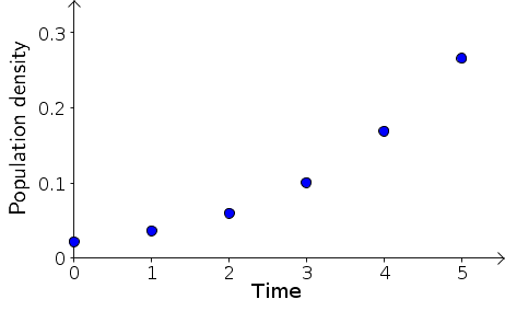
We begin by looking at the plot of bacteria density $B_t$ versus the rescaled time $t$, above. It's immediately clear that the density is increasing faster and faster as time progresses. Dynamics is all about the change in the state variables, so let's focus in on the change in $B_t$ at each time step. The population change per unit time is simply $B_{t+1}-B_{t}$. These changes are, for example, $B_1 - B_0 = 0.014$ and $B_2 - B_1 = 0.024$. Calculating all these population changes, we add them to our table of results. From now on, let's just use the rescaled time $t$.
| Time $t$ | Population Density $B_t$ | Pop Change/ $B_{t+1}\nobreak{-}B_t$ |
|---|---|---|
| 0 | 0.022 | 0.014 |
| 1 | 0.036 | 0.024 |
| 2 | 0.060 | 0.041 |
| 3 | 0.101 | 0.068 |
| 4 | 0.169 | 0.097 |
| 5 | 0.266 |
Visualizing population change versus time
We can visualize these dynamics by plotting the population change as a function of time, below. As we observed from the original plot, the population change increases as a function of time.
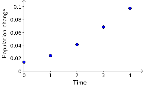
If we stare at the above plot, we can observe that the population change increases faster than linearly. In other words, the above points don't increase as a straight line, but the trail of points tends to bend upward as time increases. It doesn't look like we can make a good dynamical systems model by finding some slope $m$ and a constant $c$ and writing $B_{t+1}-B_{t}=mt+c$. Lines are one of the simplest types of equations, so we often want to find a nice simple linear relationship among variables. But, here, it looks like it won't be able to do that.
If all we had were these points and we forgot the experimental system that they came from, we might start employing some more mathematical tricks to find a nice equation for these points. We might think that, since it doesn't look like the points fall on a line, maybe they fall on a parabola. In fact, we could find an equation for a parabola that gets fairly close to these points.
But, before we start going down that road, we need to stop and remember the system we are trying to model. Our purpose in modeling the data is not simply to find an equation that matches the data points. Our goal is a model that captures the mechanism of the physical system we modeling. To achieve a model that captures the key features of bacteria population growth, we need to go back and recall what we know about how bacteria reproduce.
As mentioned at the outset, bacteria cells reproduce by dividing into two cells, and each cell takes about the same time to mature and divide. If our snapshots occurred at the same interval as this dividing time, the population size would double at each time step, as it did in the example we used to illustrate dynamical systems, captured by the bacteria doubling applet.
Looking at the above data, it doesn't appear that the population is doubling at each time step. If it doubled, we would have expected that the change $B_{t+1}-B_{t}$ would be equal to the previous population size $B_t$. In all cases, the change $B_{t+1}-B_{t}$ is substantially less than $B_t$.
What went wrong here? Let's imagine the bacteria cells are indeed dividing in half after a certain period of time. The above snapshots were taken every sixteen minutes. If each bacterium took sixteen minutes to mature and divide, then we'd expect the population to double each time step of sixteen minutes. Since the population growth seems to be slower, it's reasonable to assume each bacterium takes longer than sixteen minutes to mature and divide.
Fitting a linear model to population change versus density
If cells are taking longer than a time step to mature and divide, a reasonable assumption is that a certain fraction of the cells divide each time step. The population change, $B_{t+1}-B_{t}$, should reflect the number of cells that divided between the snapshot at time $t$ and the snapshot at time $t+1$. Therefore, if cells are dividing at a constant rate, then we expect that the population change, $B_{t+1}-B_{t}$, should be some fixed fraction of the population $B_t$. In other words, we expect that the model should be of the form \begin{gather} B_{t+1}-B_{t} = r B_t \label{constant_rate}\tag{1} \end{gather} for some constant $r$.
We can test this hypothesis by plotting the data a little differently. Instead of plotting population change versus time, as we did above, we should plot the population change, $B_{t+1}-B_{t}$, versus the population size $B_t$. If equation \eqref{constant_rate} holds, then the resulting points should lie on a line that goes through the origin. The slope of the line will give us the constant $r$, which is the fraction of the bacteria that divided in the time step.
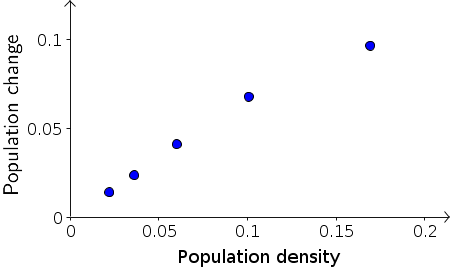
As shown in the above plot, the first four data points of population change versus density are pretty much aligned along a line through the origin. The last point doesn't seem to be exactly in line with the first four, but is a little lower. For now, let's not worry about the last point and focus on the initial growth represented by the first four points. In the following applet, you can fit the points with a line by moving the red diamond. Then, you can read off the slope, which is the constant $r$ in equation \eqref{constant_rate}.
Fitting a linear model to bacteria population change as a function of density. Bacteria population density data is plotted by the blue points in the left panel and shown as a chart in the right panel. A list of the population density $B_t$ at time $t$ is shown in the right panel along with the population change (which is $B_{t+1}-B_t$). By moving the point $P$ (represented by the red diamond) with the mouse, you can find a line through the origin that is close to most of the points and read off its slope.
From exploring the linear fit in the applet, you can observe that the first points lie along a line through the origin whose slope is approximately $2/3$. For example, if you move the point $P$ to $(0.15,0.1)$ the line through $P$ is close to the first four points, and the slope is $0.1/0.15=2/3$ (though the applet may show it as a slightly different number due to rounding). The line can be “fit” more quantitatively, but it is not necessary to do so at this stage.
In the above applet, we forced the line to go through the origin. Why did we insist the line that goes through the origin? See exercise 3.
Substituting $r=2/3$ into equation \eqref{constant_rate}, we arrive at the following evolution rule for our initial discrete dynamical system model describing bacterial population growth: \begin{gather} B_{t+1}-B_{t} = \frac{2}{3} B_t. \label{initial_model}\tag{2} \end{gather} In words equation \eqref{initial_model} says that the growth during the $t$th time interval is $\frac{2}{3}$ times $B_t$, the bacteria present at the beginning of the period. The number $\frac{2}{3}$ is called the relative growth rate, i.e., the growth per time interval is two-thirds of the current population size. More generally, one may say that a fixed fraction of cells divide every time period. (In this instance, two-thirds of the cells divide every 16 minutes.)
Solving the model
Solving a bacteria growth model.
The dynamical system of equation \eqref{initial_model} is simple enough that we can solve it to find an equation for $B_t$ in terms of $t$. As a first step, we change equation \eqref{initial_model} from difference form to function iteration form. We just rewrite equation \eqref{initial_model} so that $B_{t+1}$ is alone on the left hand side: \begin{gather} B_{t+1} = \frac{5}{3} B_t = f(B_t)\label{model_iterator}\tag{3} \end{gather} where the function $f$ is defined by $f(x)=\frac{5}{3} x$. As discussed in the introduction to discrete dynamical systems, evolving a discrete dynamical system can consist of iterating a function such as $f$.
Iterating $f$, we can calculate the values of $B_t$ given the model of equation \eqref{model_iterator}. The result will be in terms of the initial condition $B_0$. Equation \eqref{model_iterator} is shorthand for at least five equations \begin{gather*} B_1 = \frac{5}{3} B_0, \quad B_2 = \frac{5}{3} B_1, \quad B_3 = \frac{5}{3} B_2, \quad B_4 = \frac{5}{3} B_3, \quad\text{and}\quad B_5 = \frac{5}{3} B_4. \quad \end{gather*} Beginning with $B_0 = 0.022$ we can compute \begin{align*} B_1 & = \frac{5}{3} B_0 = \frac{5}{3} 0.022 \approx 0.037\\ B_2 & = \frac{5}{3} B_1 = \frac{5}{3} 0.037 \approx 0.061 \end{align*} By continuing to iterate $f$, we can compute $B_3$, $B_4$, and $B_5.$ You can do this by continuing to multiply by $5/3$ or use the function iteration applet so that you can visualize the results. To use the applet, plug in $f(x)=5x/3$ and $x_0=0.022$.
We can also write out the solution without putting in the value for the initial condition and without multiplying out the solution. In this case, the solutions look like \begin{align*} B_1 & = \frac{5}{3} B_0\\ B_2 & = \frac{5}{3} B_1 = \frac{5}{3} \times \left( \frac{5}{3}\, B_0 \right) = \frac{5}{3} \times \frac{5}{3} B_0 \\ B_3 & = \frac{5}{3} B_2 = \frac{5}{3} \times \left(\frac{5}{3} \times \frac{5}{3} B_0 \right) = \frac{5}{3} \times \frac{5}{3} \times \frac{5}{3} B_0 \end{align*}
At time interval 5, we get \begin{align*} B_5 = \frac{5}{3} \times \frac{5}{3} \times \frac{5}{3} \times \frac{5}{3} \times \frac{5}{3} \times B_0 \end{align*} which is cumbersome and is usually written \begin{align*} B_5 = \left( \frac{5}{3} \right)^5 \times B_0. \end{align*} The general form is \begin{equation} B_t = \left( \frac{5}{3} \right)^t B_0 = B_0 \left( \frac{5}{3} \right)^t \label{general_solution}\tag{4} \end{equation} which is the general solution to the discrete dynamical system \eqref{initial_model} for generic initial conditions $B_0$.
For the data, we had the specific initial population density $B_0 = 0.022$. For that situation, equation \eqref{general_solution} becomes \begin{equation} B_t = 0.022 \left( \frac{5}{3} \right)^t \label{specific_solution}\tag{5} \end{equation} and is the specific solution to the discrete dynamical system of equation \eqref{initial_model} and the given initial condition, which we rewrite together as \begin{gather*} B_0 = 0.022, \qquad B_{t+1} - B_t = \frac{2}{3} B_t. \end{gather*}
Equation \eqref{specific_solution} is written in terms of the time index, $t$. We can also write the solution in terms of original experimental time. Denoting this time in minutes by $T$, where $T=16 t$, we can write equation \eqref{specific_solution} as \begin{gather} \text{Bacteria at $T$ minutes} = 0.022 \left( \frac{5}{3} \right)^{T/16}\goodbreak \approx 0.022 \timesbadbreak 1.032^T. \label{specific_solution_time_units}\tag{6} \end{gather}
How well did we do?
How well do the computed values of bacterial density, $B_t$, match the observed values? The original and computed values are shown in the following table.
| Time (min) | Time index | Population Density | Computed Density |
|---|---|---|---|
| 0 | 0 | 0.022 | 0.022 |
| 16 | 1 | 0.036 | 0.037 |
| 32 | 2 | 0.060 | 0.061 |
| 48 | 3 | 0.101 | 0.102 |
| 64 | 4 | 0.169 | 0.170 |
| 80 | 5 | 0.266 | 0.283 |
To visualize the comparison, we can plot the values computed from the along with the data. You can use the following applet to create such a plot. The applet allows you to compare model values for different values of the growth parameters. If you like to think of the model in difference form, you can enter $r=2/3$ in the applet to reproduce the obtain model fit written as equation \eqref{initial_model}. Equivalently, if you prefer function iteration form, you could obtain the results by entering $R=5/3$, as in equation \eqref{model_iterator}.
Bacteria density versus time along with exponential growth fit. The growth of the bacteria population density is compared with an exponential growth model. The data is displayed by the blue circles. The exponential growth model can be either written in difference form as $$B_{t+1} - B_t = r B_t$$ or in function iteration form as $$B_{t+1} = R B_t,$$ where the two growth parameters related by $R=r+1$. You can change either growth parameter $r$ or $R$ by typing a value in the corresponding box. The other parameter will be updated automatically. The model results are are displayed by the red crosses. For a certain value $r$ or $R$, the model results should fit the data fairly closely.
If you enter $r=2/3$ or $R=5/3$, the computed model values match the observed values closely except for the last measurement where the observed value is less than the value predicted from the mathematical model. The effect of cell crowding or environmental contamination or age of cells is beginning to appear after an hour of the experiment and the model does not take this into account. We will return to this population with data for the next 80 minutes of growth later and will develop a new model that will account for decreasing rate of growth as the population size increases.
To learn how to build your own dynamical system models, try your hand at the exercises.
Thread navigation
Elementary dynamical systems
Math 1241, Fall 2020
- Previous: Online quiz: Quiz 2
- Next: Bacteria growth model exercises
Math 201, Spring 22
- Previous: Online quiz: Quiz 2
- Next: Bacteria growth model exercises
Similar pages
- Bacteria growth model exercises
- Bacteria growth model exercise answers
- Environmental carrying capacity
- Developing a logistic model to describe bacteria growth
- Harvest of natural populations
- Harvest of natural populations exercises
- Harvest of natural populations exercise answers
- The idea of a dynamical system
- An introduction to discrete dynamical systems
- Exponential growth and decay modeled by discrete dynamical systems
- More similar pages