Developing a logistic model to describe bacteria growth
Introduction
Developing a logistic model to describe bacteria growth, introduction.
When we modeled the initial growth of the bacteria V. natriegens, we discovered that an exponential growth model was a good fit to the first 64 minutes of the bacteria growth data. However, the last data point at 80 minutes was lower that predicted by the exponential growth model. It appeared that the growth rate was slowing down during the last 16 minutes of that data set. A likely explanation is that the population was beginning to exhaust its environment.
The logistic growth model is a model that includes an environmental carrying capacity to capture how growth slows down when a population size becomes so large that the resources available become limited. Our goal is to apply this model to the bacteria growth data to see if the pattern in the data can be explained by such a model. Fortunately, we have more data than we revealed in the initial bacteria model page. We actually have data from growing V. natriegens in a flask for 160 minutes, as shown in the following table. The population was measured every 16 minutes, and the time index variable $t$ measures the number of these 16 minute intervals since the beginning of the experiment.
| Time (min) | Time index $t$ | Population Density |
|---|---|---|
| 0 | 0 | 0.022 |
| 16 | 1 | 0.036 |
| 32 | 2 | 0.060 |
| 48 | 3 | 0.101 |
| 64 | 4 | 0.169 |
| 80 | 5 | 0.266 |
| 96 | 6 | 0.360 |
| 112 | 7 | 0.510 |
| 128 | 8 | 0.704 |
| 144 | 9 | 0.827 |
| 160 | 10 | 0.928 |
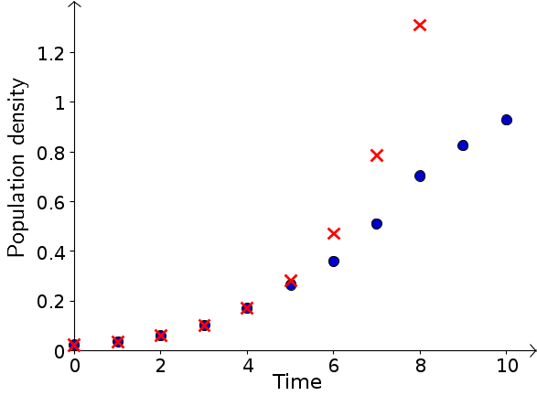
When fitting an exponential growth model to the data from the first 5 intervals, we discovered that a relative growth rate of $r=2/3$ described the first four data points well. If we let $P_t$ be the population density in time bin $t$, then the initial model (equation (2) of the initial model page) was \begin{gather*} P_{t+1}-P_{t} = \frac{2}{3} P_t. \end{gather*} For the fifth point, however, the data was a little lower than the model prediction. If the population growth rate is slowing down, we expect the discrepancy between the model prediction and the data to get even worse for later times. As shown in the below figure, this expectation is born out. The data is shown by the blue circles and the model prediction by the red X's. For the sixth time point and beyond, the exponential growth model grossly overestimates the population size.
This deviation between the data and the model bears a reasonable resemblance to the comparison between logistic and exponential growth that we observed when modeling the effects of environmental carrying capacity. We will look for a logistic equation that approximates the V. natriegens data. The equation should be of the form \begin{equation} \label{logistic} P_{t+1} - P_t = r P_t \left(1 - \frac{P_t}{M} \right). \end{equation} In order to use such a discrete dynamical system model, we must have an initial value, $P_0$, which we can take directly from the data. The more challenging task will be to find reasonable values for the low density growth rate $r$ and the carrying capacity $M$.
To accomplish this task, we are going to use Geogebra. Although it might be possible to accomplish the task using the below applet as embedded in this web page, it will be a lot easier if you download the Geogebra program onto your own computer. Then, from the bacteria density data applet page (which you can also view by clicking on “More information about applet” in the applet's caption) download the applet file and open it in Geogebra. In this way, you can save or print your work and will have more options available to work with.
Bacteria density data. An applet where you can explore different features of the data consisting of the population density of the bacteria V. natriegens as measured every 16 minutes for 160 minutes. Click “More information about applet,” below, to view the applet page for instructions on how to download the applet file and open it in Geogebra on your own computer.
Trying the old method: plotting population change versus density
The following video explains how to use the Geogebra applet to attempt to fit an exponential growth model to the bacteria data. (It shouldn't fit the data very well.) The instructions are also written out below the video.
Developing a logistic model to describe bacteria growth, old method.
In developing the exponential model for bacteria growth, a critical step was to plot the population change $P_{t+1}-P_t$ in one time interval versus the population density $P_t$ at the beginning of the interval. By fitting the resulting data points by a line through the origin, we obtained the growth rate $r$ as the slope of the line. What would happen if we attempted to follow this procedure with the full bacteria growth data?
Using the bacteria density data applet file that you are running from within Geogebra installed on your computer, create a plot of population change $P_{t+1}-P_t$ versus population density $P_t$ and see if the data is well fit by a line through the origin. Use the spreadsheet panel to calculate the population change $P_{t+1}-P_t$ as follows.
Create a column to the right of the data with a heading such as “change.” You can let the spreadsheet calculate the differences for you. For example, in cell D2, type “=”, click the C3 cell (which is $P_1$), type “-”, click the C2 cell (which is $P_0$), then press Enter. If all goes well, cell D2 should then contain $P_1-P_0$, which is 0.014. You can repeat this procedure for the remaining cells in the column or save yourself work by copying and pasting the result into the rest of the column. (The copy and paste keys, Ctrl+C and Ctrl+V, won't work in the applet when it's embedded in the web page. You'd need to select D2 and drag the little square that appears in the lower right corner of the cell to extend the formula to the rest of the column.)
If you copy the formula to the last row corresponding to time index 10, Geogebra will automatically insert a 0 in the population column of the following row, giving a population density of zero in time index 11 (i.e., $P_{11}=0$) and a negative change for $P_{11}-P_{10}$. Keeping that negative change around will mess up the data analysis, so be sure to delete it if you inadvertently create it.
To plot points in the graphics panel at the left from the data in the spreadsheet, there is a trick. If a spreadsheet cell contains data of the form $(x,y)$, where $x$ and $y$ are numbers, then Geogebra will plot a point at the coordinates $(x,y)$ in the graphics panel. According to our analysis with the exponential bacteria growth model, if we plot the change versus population size, the exponential growth model predicts the points should lie on along a line through the origin. To test the validity of this model plot the values $P_{t+1}-P_{t}$ that you just calculated in column D versus the population size in column C. Create the points in column E. If you like you can type a label for the column in cell E1. Then, type “=(” in cell E2, click cell C2, type “,”, click cell D2, and press Enter. (You don't have to type the final “)” as Geogebra can add that in for you.) Copy cell C2 to the rest of column C, and you should see the points $(P_{t},P_{t+1}-P_{t})$ appear in the graphics panel, similar to how they are shown in the applet used for initial bacteria data.
If you don't like the labels such as E2 to appear, you can highlight the points either in the graphics window or the spreadsheet, right-click (Mac OS: Ctrl-click) and select Object Properties. In the Basic tab, unselect Show Label. You can also change the color and style of the points from this dialog box, if you like.
What do you observe about the pattern of the points $(P_{t},P_{t+1}-P_t)$? Explain how this plot informs you about the growth rate of the bacteria.
A new approach: plotting relative population change
The following video shows the steps necessary to fit a logistic model to the bacteria data. The video explains just the mechanics for working with the Geogebra applet. The text below the video details how the calculations from the Geogebra applet relate to the logistic model and explains how to obtain the logistic model parameters from the data fitting.
Developing a logistic model to describe bacteria growth, new method.
According to the exponential growth dynamical system $$P_{t+1}-P_{t}=rP_t,$$ the change $P_{t+1}-P_{t}$ is proportional to the population density $P_t$ with proportionality constant $r$. In other words, the population change $P_{t+1}-P_{t}$ relative to the the population size $P_t$ is held constant: $$\frac{P_{t+1}-P_{t}}{P_t}=r.$$
The idea of an environmental carrying capacity is that this relative population change is reduced as the population size increases, approaching zero as the carrying capacity is reached. For the logistic model of equation \eqref{logistic}, the relative population change is proportional to the unused carrying capacity \begin{align} \frac{P_{t+1}-P_{t}}{P_t}=r \left(1 - \frac{P_t}{M} \right), \label{logistic_relative_change} \end{align} as discussed on the environmental carrying capacity page.
We can use this relation to fit the logistic growth model to the bacteria data. All we need to do is plot the relative population change $(P_{t+1}-P_{t})/P_t$ versus the population size $P_t$. If we let $x=P_t$ and $y=(P_{t+1}-P_{t})/P_t$, then equation \eqref{logistic_relative_change} becomes \begin{align*} y &= r\left(1 - \frac{x}{M} \right)\\ &= r - \frac{r}{M}x. \end{align*} The data should lie along a line of with slope $-r/M$ and $y$-intercept $r$.
Test to see if a plot of relative change versus population density do lie approximately along a line with negative slope. Follow the procedure in the above video to create the points. Briefly the procedure is to calculate in one column, say column F, the relative population change as the ratio of the change to the population density. This column will be the $y$ values defined above. The $x$ values will be the population size from column C. In another column, say column G, create the points $(x,y)$ from the values in column C and F. (If you still have the old points from the previous model in column E, you can delete the old points or hide them by highlighting column E, right clicking (Mac OS: Ctrl-clicking), selecting Object Properties, and clearing the Show Object box in the Basic tab.)
Do the points seem to lie approximately along a line with negative slope? There should be plenty of scatter, as the data comes from an actual experiment. How do we fit a line through the data so that we can estimate the slope and $y$-intercept? We could, as we did before, just fit a line by eye. But, especially since we need to fit two parameters, there will be too much wiggle room to find the best line. Instead, we'll let Geogebra fit a line through the data.
You can let Geogebra fit the line in two ways. In Input box at the bottom, you could type (assuming your points are in column G):
FitLine[{ G2, G3, G4, G5, G6, G7, G8, G9, G10, G11}]
You can also use the ![]() Best Fit Line tool in Geogebra.
Best Fit Line tool in Geogebra.
If you did this right, you should have a line that fits the data reasonably well. Now, you just need to read off the slope and $y$-intercept. Unfortunately, it's not as easy as right-clicking (Mac OS: Ctrl-clicking) the line and viewing its properties.
You have two ways of determining the slope and intercept. One way is to open the Algebra window. Select Algebra from the View menu. In the Algebra window, the equation for the line will be displayed in terms of the variables $x$ and $y$. You can use the equation to calculate the slope and $y$-intercept. Alternatively, you can use the ![]() Slope tool to determine the slope of the line. Then, you can use the
Slope tool to determine the slope of the line. Then, you can use the ![]() Intersect Two Objects tool to find the intersection between the line and the $y$-axis, the $y$-coordinate of which is the $y$-intercept of the line.
Intersect Two Objects tool to find the intersection between the line and the $y$-axis, the $y$-coordinate of which is the $y$-intercept of the line.
The $y$-intercept of your linear fit to the data gives your estimate of the low density growth rate $r$. The slope of the line is your estimate of $-r/M$, from which you can estimate carrying capacity $M$. According to our model, the low density growth rate $r$ from the logistic model should be similar to the growth rate $r$ that we obtained for the exponential growth fit to the initial data. We obtained $r=2/3$ for the exponential growth fit. Is your estimate of the low density growth rate $r$ of the logistic model similar to this value of $2/3$?
If the bacteria population were really exhibiting exponential growth, what would the plot of $y=(P_{t+1}-P_{t})/P_t$ versus $x=P_t$ look like? Supposedly, the first four points were pretty close to the exponential growth model. Could the first four points on your graph be well fit by this prediction from the exponential growth model?
Comparing model prediction to the data
Now that you have determined the low density growth rate $r$ and the carrying capacity $M$ from the data, let's see how well the logistic model \eqref{logistic} fits the data. We'll use the initial condition $P_0 = 0.022$ from the first data point. Calculate the remaining $P_t$ as predicted from the logistic model and see how you did. The above video describes a procedure for using the applet to create such a plot. This procedure is summarized here.
First, hide (or delete) any the points from a previous plot. Then, create a column with points $(x,y)$ where $x$ is the time index (column B) and $y$ is the population size (column C). To see these points, you'll need to rescale the $x$-axis. One way to do so is hold down the Shift key while dragging on the $x$-axis with your mouse. You can also right-click (Mac OS: Ctrl-click) the background of the graphics panel and select Graphics to enter the dimensions of the graphics panel directly.
You can easily create the logistic model predictions in the spreadsheet as well. Label a new column with something like “model” and copy the first entry from Population column as the initial condition. In the cell immediately below, type “=” and then the formula \eqref{logistic}, only solve it for $P_{t+1}$ first. In every instance of $P_t$ click on the cell where you entered the initial condition. Enter your calculated values for the parameters $r$ and $M$. When you are done, you should have calculated $P_1$ based on the logistic model and $P_0$. Simply copy this formula to the rest of the column, and the spreadsheet will automatically calculate future values. Be sure to go all the way down to the row with time index $t=10$ (i.e., row 12). Then, in the column to the right, you can create points $(x,y)$, where $x$ is the time index and $y$ is your newly calculated model predictions. You can select those points, remove their labels, and change their color and style so they look different from the actual data points.
How did the model do? Do the model points match well with the data points? Does it seem like the slowing growth rate in the data can be well modeled by the carrying capacity as incorporated into the logistic growth equation?
Project
The bacteria logistic growth project page gives instructions for writing up a project report based on this exploration.
Thread navigation
Elementary dynamical systems
- Previous: Environmental carrying capacity
- Next: Project: Project on developing a logistic model to describe bacteria growth
Math 1241, Fall 2020
- Previous: Environmental carrying capacity
- Next: Project: Project on developing a logistic model to describe bacteria growth
Math 201, Spring 22
Similar pages
- Developing an initial model to describe bacteria growth
- Bacteria growth model exercises
- Bacteria growth model exercise answers
- Environmental carrying capacity
- Harvest of natural populations
- Harvest of natural populations exercises
- Harvest of natural populations exercise answers
- The idea of a dynamical system
- An introduction to discrete dynamical systems
- Exponential growth and decay modeled by discrete dynamical systems
- More similar pages