The arc length of a parametrized curve
A vector-valued function of a single variable, $\dllp: \R \to \R^n$ (confused?), can be viewed as parametrizing a curve. Such a function $\dllp(t)$ traces out a curve as you vary $t$.
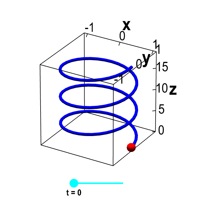
You could think of a curve $\dllp : \R \to \R^3$ as being a wire. For example, $\dllp(t) = (\cos t, \sin t, t)$, for $0 \le t \le 6\pi$, is the parametrization of a helix. You can view it as a slinky or a spring.
Applet loading
Parametrized helix. The vector-valued function $\dllp(t)=(\cos t, \sin t, t)$ parametrizes a helix, shown in blue. This helix is the image of the interval $[0,6\pi]$ (shown in cyan) under the mapping of $\dllp$. For each value of $t$, the red point represents the vector $\dllp(t)$. As you change $t$ by moving the cyan point along the interval $[0,6\pi]$, the red point traces out the helix.
Imagine we wanted to estimate the length of the slinky, which we call the arc length of the parametrized curve. Unfortunately, it's difficult to calculate the length of a curved piece of wire. It's much easier to calculate the length of straight pieces of wire. Probably the easiest way to calculate the length of the slinky would be to stretch it out into one straight line. But, if you ever tried to do that with a slinky (or a strong spring), you'd discover that stretching it into a straight line is virtually impossible.
If you can't stretch the slinky into one straight line, what could you do to estimate its length? One thing you could do is pretend that the slinky, rather than being a curved wire, was really composed of a bunch of short straight wires. In other words, you could approximate the curved slinky with line segments.
Helix arc length. The vector-valued function $\dllp(t)=(\cos t, \sin t, t)$ parametrizes a helix, shown in blue. The green lines are line segments that approximate the helix. The discretization size of line segments $\Delta t$ can be changed by moving the cyan point on the slider. As $\Delta t \to 0$, the length $L(\Delta t)$ of the line segment approximation approaches the arc length of the helix from below.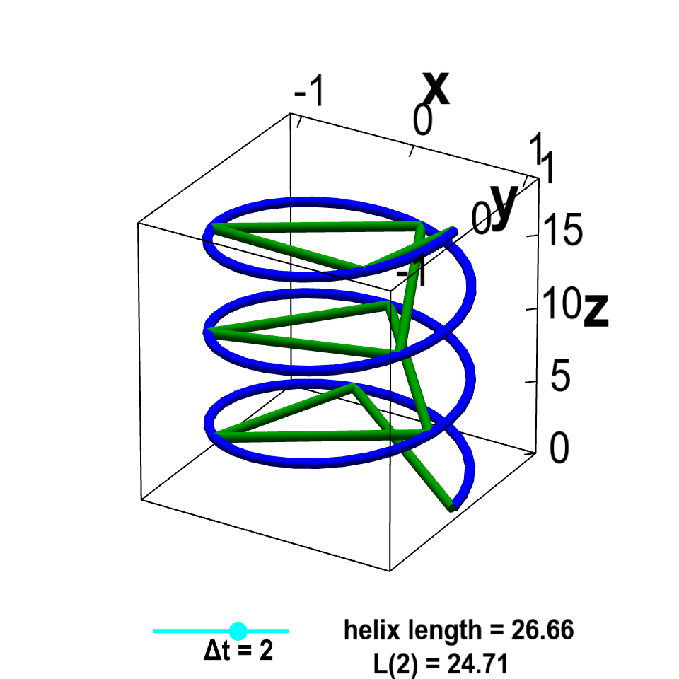
Applet loading
The length of the line segments is easy to measure. If you add up the lengths of all the line segments, you'll get an estimate of the length of the slinky. Let $\Delta t$ specify the discretization interval of the line segments, and denote the total length of the line segments by $L(\Delta t)$. As the line segments take shortcuts, the length of the line segments underestimate the arc length of the slinky.
However, if you increase the number of line segments (decreasing the length of each line segment), the total length of the line segments becomes a better estimate of the slinky arc length. As $\Delta t$ approaches zero, the length of each line segment shrinks toward zero, the number of line segments increases, and the line segments become closer and closer to the slinky. Consequently, the total length $L(\Delta t)$ of the line segments approaches the slinky arc length.
What's the length of each line segment? If there are $n$ line segments, we could define $t_0, t_1, \ldots, t_n$ so that the first line segment goes from the point $\dllp(t_0)$ to the point $\dllp(t_1)$, the second line segment goes from the point $\dllp(t_1)$ to the point $\dllp(t_2)$, etc. The vector from $\dllp(t_0)$ to $\dllp(t_1)$ is simply $\dllp(t_1) - \dllp(t_0)$, so the length of the line segment must be $\| \dllp(t_1) - \dllp(t_0) \|$. The length of the second line segment is $\| \dllp(t_2) - \dllp(t_1) \|$, etc.
To find the total length of the line segments, we just add up those lengths from all $n$ line segments: \begin{align*} \sum_i^n \| \dllp(t_i) - \dllp(t_{i-1})\|. \label{totallengtha} \end{align*}
Now we do some tricks to put this into a different form. First, if $\Delta t_i = t_i - t_{i-1}$, then we can rewrite $t_{i}$ as $t_{i-1} + \Delta t_i$. Next, we can divide each term of the above equation by $\Delta t_i$ and multiply it by $\Delta t_i$ so that our expression for the length becomes \begin{align} \sum_i^n \| \dllp(t_i) - \dllp(t_{i-1})\| &= \sum_i^n \| \dllp(t_{i-1} + \Delta t_i) - \dllp(t_{i-1})\| \notag \\ &= \sum_i^n \left\| \frac{\dllp(t_{i-1} + \Delta t_i) - \dllp(t_{i-1})}{\Delta t_i}\right\| \Delta t_i. \label{total_length} \end{align}
Maybe this new equation doesn't look like much of an improvement. But if you were a real math nerd, you might have noticed that the quotient involving $\dllp(t_{i-1})$ is exactly the expression used in the limit definition of the derivative $\dllp'(t)$ of a parametrized curve (if we replace $h$ with $\Delta t_i$). In fact, equation \eqref{total_length} is a Riemann sum for an integral, analogous to the ones used to define integrals such as double integrals. If we let the number of line segments increase (as we take the limit $\Delta t_i \to 0$) the quotient becomes $\dllp'(t)$, and equation \eqref{total_length} approaches the integral \begin{align*} L(\dllp)=\int_a^b \| \dllp'(t) \| dt, \label{totallengthc} \end{align*} which is the true arc length of the slinky. The numbers $a$ and $b$ are the values of $t$ at the ends of the slinky (i.e., the numbers so that the slinky is defined by $\dllp(t)$ for $a \le t \le b$). In our example, the slinky was defined by $\dllp(t)$ for $0 \le t \le 6\pi$, so we would use $a=0$ and $b=6\pi$.
The magnitude of the derivative $\| \dllp'(t) \|$ is the speed of a particle that is at position $\dllp(t)$ at time $t$. The above equation simply says that the total length of the curve traced by the particle is the integral of its speed. (This length must, of course, be independent of the particle's speed.)
You can see some examples here.
Thread navigation
Multivariable calculus
- Previous: Orienting curves
- Next: Parametrized curve arc length examples
Math 2374
- Previous: Triple integral examples
- Next: Parametrized curve arc length examples
Notation systems
Similar pages
- Introduction to a line integral of a scalar-valued function
- Line integrals are independent of parametrization
- Examples of scalar line integrals
- Introduction to a line integral of a vector field
- Length of curves
- An introduction to parametrized curves
- Derivatives of parameterized curves
- Tangent lines to parametrized curves
- Tangent line to parametrized curve examples
- Parametrized curve and derivative as location and velocity
- More similar pages