Math Insight

Solving single autonomous differential equations using graphical methods

Video introduction

Overview

One can understand an autonomous differential equation of the form \begin{align} \diff{x}{t} &= f(x)\\ x(t_0) &= x_0\notag \end{align} by using a purely graphical approach. We can determine the essential behavior of the solution $x(t)$ without doing any analytic calculations. A graph of the function $f(x)$ will tell us all we need to know to estimate what the solution $x(t)$ will do for any initial condition $x_0$.

Since the derivative $\diff{x}{t}$ is the rate of change of $x(t)$, a glance at the graph of $f(x)$ will tell us where $x(t)$ is increasing or decreasing and how fast it is changing. The state variable $x(t)$ moves to larger values when $f(x)$ is positive, and it moves to smaller values when $f(x)$ is negative. The velocity of $x(t)$ drops to zero when $f(x)$ reaches zero. The points where $f(x)=0$ are the equilibria where $x(t)$ does not move.

An example

For example, we'll look at the differential equation \begin{align*} \diff{x}{t} = x^2-4. \end{align*} We can determine the dynamics of the solution $x(t)$ by looking at the graph of $f(x)=x^2-4$.

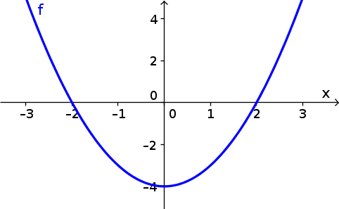
From the graph we see that $f(x) < 0$ for $x \in (-2,2)$. The rate of change $\diff{x}{t}$ must be negative for $-2 \lt x(t) \lt 2$, so the solution decreases in that range. If the initial condition $x_0$ were in the range $x_0 \in (-2,2)$, then the solution would start out decreasing. The speed of this negative change would be greatest when $x(t)=0$, and then the trajectory would slow down as it got closer to $x(t)=-2$.

The function $f(x)$ is zero at $x=2$ and $x=-2$. Therefore, these two values of $x(t)$ are equilbria. If the initial condition $x_0$ were $x_0=-2$, then the solution would be a constant $x(t)=-2$ for all time. Similarly, if the initial condition were $x_0=2$, then the solution would be the constant $x(t)=2$ for all time. For the case mentioned above, with initial condition $x_0 \in (-2,2)$, the trajectory would get closer and closer to $-2$. It could never cross $x=-2$ because we know the velocity is zero at that point.

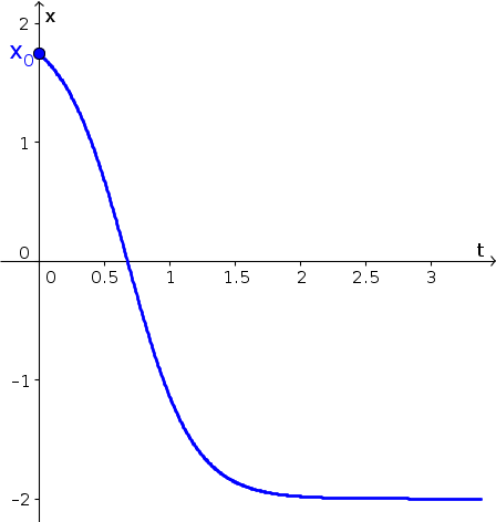
One solution to an initial condition just below 2 is graphed below. In the graph, $x(t)$ is plotted as a function of $t$. In this plot, the $x$-axis has moved to the vertical axis, and the $t$-axis is the horizontal axis. Notice that $x(t)$ decreases the whole time, decreases most quickly around $x=0$, then slows down, getting closer and closer to $x=-2$ as the time $t$ increases.

What changes if the initial condition is below $x=-2$. In that case, the function $f(x)$ is positive, so the rate of change $\diff{x}{t}$ is positive. If the initial condition $x_0 \lt -2$, then the solution $x(t)$ starts out increasing. If $x_0$ is much smaller than $-2$, then $x(t)$ increases very quickly, but its velocity slows down as $x(t)$ approaches the equilibrium $x=-2$. It continues to increase the whole time, as it can't cross the equilibrium, but its velocity goes to zero as it gets closer to the equilibrium.

The graph of $f(x)$ is symmetric across the vertical axis. So, it might seem that something similar will happen for initial conditions above the upper equilibrium $x=2$. However, the behavior is entirely different. Just as in the case for $x_0 \lt -2$, for initial condition $x_0 \gt 2$, the trajectory starts off with a positive rate of change $\diff{x}{t}$. In this case, though, as $x(t)$ increases, its velocity increases even more. The trajectory quickly blows up to very large values.

In the following applet, you can explore the behavior of solutions to $\diff{x}{t} = x^2-4$ for many different initial conditions. You can observe how initial conditions below $x=2$ lead to solutions $x(t)$ that converge toward $x=-2$. You can also see how quickly solutions with initial conditions $x_0 \gt 2$ blow up. This applet will also help you solidify the relationship between the graph of $f(x)$ (where $x$ is the horizontal axis) and the graph of the trajectories versus time (where $x$ is the vertical axis).

The second applet lets you see the simultaneous behavior of six solutions with different initial conditions. Before you hit play or move the $t$ slider, see if you can predict what the solutions will look like.