Introduction to a line integral of a scalar-valued function
A line integral (sometimes called a path integral) of a scalar-valued function can be thought of as a generalization of the one-variable integral of a function over an interval, where the interval can be shaped into a curve. A simple analogy that captures the essence of a scalar line integral is that of calculating the mass of a wire from its density.
If the density of a wire were constant, then one could calculate its mass by multiplying the density by the arc length of the curve. If, on the other hand, the density varies along the wire, one can use a procedure similar to that of calculating the arc length to derive a formula for the density. This formula defines of the line integral over the wire of the function giving the density.
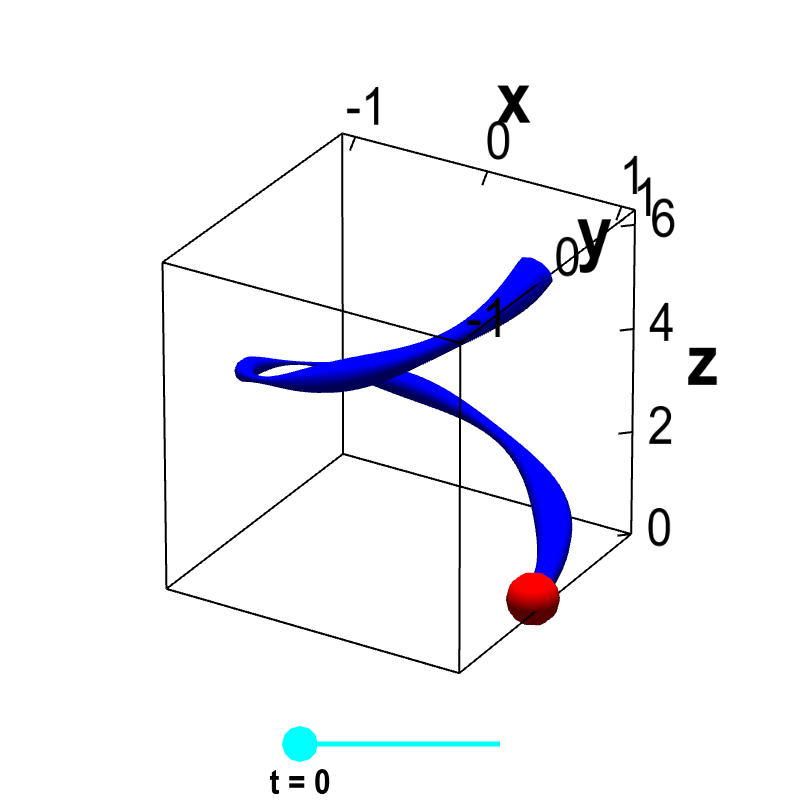
Extending the slinky example used to introduce arc length, we let one coil of the slinky be parametrized by $\dllp(t) = (\cos t, \sin t, t)$, for $0 \le t \le 2\pi$, and imagine that the density of the slinky at the point $(x,y,z)$ is given by some function $\dlsi(x,y,z)$. This function describes how the slinky might be thicker in some parts and thinner in others. For a given value of $t$, a point on the slinky is $\dllp(t)$, and the density of the slinky at that point is $\dlsi(\dllp(t))$, as illustrated below.
Applet loading
Helix with variable density. The function $\dllp(t) = (\cos t, \sin t, t)$, for $0 \le t \le 2\pi$ parametrizes a helix. The blue curve representing the helix is drawn with a variable width, representing the varying density $\dlsi(x,y,z)$ of the helix at each point $(x,y,z)=\dllp(t)$ along its length. By dragging the cyan point representing $t$ on the slider, one can move the red point $\dllp(t)$ along the helix.
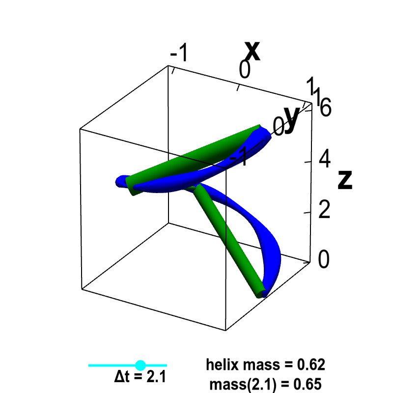
To calculate the mass of the slinky, we repeat the procedure we used to calculate its length. We pretend the slinky is composed by a bunch of straight line segments. Moreover, we assume each line segment has constant density, so the mass of the line segment is simply its length times its density. We let the density of each line segment be the density of the slinky at the point where the upper end of the line segment touches the slinky. (In the below applet, we use width of the curves to represent density.) For a given discretization $\Delta t$, we estimate the mass of the slinky as the total mass of the line segments (labeled as mass($\Delta t$)).
Applet loading
Line integral of helix mass from density. The function $\dllp(t) = (\cos t, \sin t, t)$, for $0 \le t \le 2\pi$ parametrizes a helix. The blue curve representing the helix is drawn with a variable width, representing the varying density $\dlsi(x,y,z)$ of the helix at each point $(x,y,z)=\dllp(t)$ along its length. The green line segments of constant width represent segments of constant density that approximate the helix. The discretization size of the line segments $\Delta t$ can be changed by moving the cyan point on the slider. As $\Delta t \to 0$, the mass of the line segment approximation, labeled mass($\Delta t$), approaches the actual mass of the helix.
We can increase the number of line segments (decreasing the length of each line segment) so that the total mass of the line segments becomes a better estimate of the slinky mass. As the discretization size $\Delta t$ approaches zero, the length of each line segment shrinks toward zero, the number of line segments increases, and the density of each line segment more closely approximates the density of the slinky. Since the total length of the line segments approaches the slinky length, the total mass of the line segments approaches the mass of the slinky.
The derivation of the line integral formula is similar to the procedure we used to estimate the slinky length. The length of the $i$th line segment can be written as $\|\dllp(t_i) - \dllp(t_{i-1})\|$. The density of the line segment is simply $\dlsi(\dllp(t_i))$ since $\dllp(t_i)$ is the point where the upper end of the line segment touches the slinky. The mass of the line segment is its density times its length: $\dlsi(\dllp(t_i))\|\dllp(t_i) - \dllp(t_{i-1})\|$. We obtain the total mass of the line segments by summing over all $n$ line segments: \begin{align*} \sum_i^n \dlsi(\dllp(t_i)) \| \dllp(t_i) - \dllp(t_{i-1})\|. \end{align*}
The only difference between the above expression and the one we obtained for arc length calculation is the $\dlsi(\dllp(t_i))$ factor. To turn this into an integral, we repeat the same steps we did on that page. We again let $\Delta t_i = t_i - t_{i-1}$, multiply and divide each term by $\Delta t_i$, and obtain the more complicated looking expression. \begin{align*} \sum_i^n \dlsi(\dllp(t_i))\| \dllp(t_i) - \dllp(t_{i-1})\| &= \sum_i^n\dlsi(\dllp(t_i)) \left\| \frac{\dllp(t_{i-1} + \Delta t_i) - \dllp(t_{i-1})}{\Delta t_i}\right\| \Delta t_i. \end{align*} Since the ugly expression in the $\| \cdot \|$ is the quantity in limit definition of the derivative of $\dllp(t)$, when we let $\Delta t_i \to 0$ and $n \to \infty$, the above Riemann sum converges to the integral \begin{align*} \int_a^b \dlsi(\dllp(t))\| \dllp\,'(t) \| dt, \end{align*} where $a=0$ and $b=2\pi$. This is called the line integral of $\dlsi$ over the curve parametrized by $\dllp$.
We often use $\als(t)$ to be the length of the slinky from the beginning point $\dllp(a)$ up to the point $\dllp(t)$. If you think of $d\als$ as being the length of a tiny line segment approximating the slinky, then the mass of that tiny line segment is $\dlsi$ times $d\als$. For this reason, we often denote the integral representing the mass of the slinky as \begin{align*} \slint{\dllp}{\dlsi} =\int_a^b \dlsi(\dllp(t))\| \dllp\,'(t) \| dt. \end{align*}
The notation $\slint{\dllp}{\dlsi}$ indicates that the integral of $\dlsi$ is over the parametrized curve $\dllp$. But, if the integral can really represent the mass of a wire with density $\dlsi$, then the mass should not depend on how we chose to parametrize the wire. In fact, it does not, and you can read about how the line integral is independent of the parametrization used to represent the curve.
You can also read some examples of calculating line integrals of scalar functions.
Thread navigation
Multivariable calculus
- Previous: Calculating the formula for circulation per unit area
- Next: Introduction to a line integral of a vector field
Math 2374
Notation systems
Similar pages
- Line integrals are independent of parametrization
- Examples of scalar line integrals
- Introduction to a line integral of a vector field
- The arc length of a parametrized curve
- Alternate notation for vector line integrals
- Line integrals as circulation
- Vector line integral examples
- The integrals of multivariable calculus
- Length of curves
- An introduction to parametrized curves
- More similar pages