An introduction to parametrized curves
A simple way to visualize a scalar-valued function of one or two variables is through their graphs. In a graph, you plot the domain and range of the function on the same set of axes, so the value of the function for a value of its input can be immediately read off the graph. Whether you plot the function $f(x)$ by the curve of points $(x,f(x))$ or the function $f(x,y)$ by the surface of points $(x,y,f(x,y))$, these graphs give a fairly comprehensive view of the behavior of the function.
If we have a two-dimensional vector-valued function of a single variable, $\vc{f}: \R \to \R^2$ (confused?), it is still possible to display its graph. If the function is $\vc{f}(t)=(f_1(t),f_2(t))$, we could plot the set of points $(t,f_1(t),f_2(t))$ and obtain a curve in three-dimensional space.
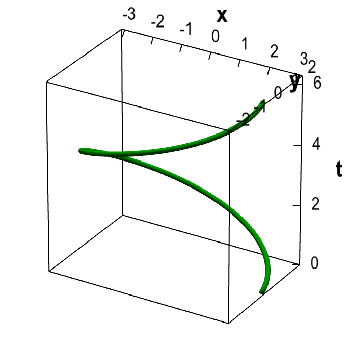
For example, the graph of the function $\dllp(t)=(3\cos t)\vc{i} + (2 \sin t) \vc{j}$ is a spiral, or helix, as shown here.
Applet loading
Graph of a function that parametrizes an ellipse. The green curve is the graph of the vector-valued function $\dllp(t) = (3\cos t, 2\sin t)$. This function parametrizes an ellipse. Its graph, however, is the set of points $(t,3\cos t, 2\sin t)$, which forms a spiral.
Graphing a vector valued function is possible for functions $\vc{f}: \R \to \R^2$ because the graph required only three dimensions. However, we are unable to plot the graph with an higher-dimensional input or output space, as these graphs would require more than three dimensions. We need a new method to visualize these functions.
One way to visualize vector-valued functions is by choosing a set in their domain and viewing how the function maps this set into its range. This procedure is particularly effective for vector-valued functions of a single variable. We pick an interval in their domain, and these functions will map that interval into a curve. If the function is two or three-dimensional, we can easily plot these curves to visualize the behavior of the function.
Returning to the example function $\dllp(t)=(3\cos t)\vc{i} + (2 \sin t) \vc{j}$, you can see in the below applet how it maps the interval $[0,2\pi]$ into an ellipse. As $t$ sweeps through the interval $[0,2\pi]$, the vector $\dllp(t)$ sweeps out the ellipse. We refer to $t$ as a free parameter, and say that $\dllp$ parametrizes the ellipse. (You can see the applet's page for details on how to show that $\dllp$ indeed sweeps out a ellipse.)
Parametrized ellipse. The vector-valued function $\dllp(t)=(3\cos t)\vc{i} + (2 \sin t) \vc{j}$ parametrizes an ellipse, shown in green. This ellipse is the image of the interval $[0,2\pi]$ (shown in red) under the mapping of $\dllp$. For each value of $t$, the blue vector is $\dllp(t)$. As you change $t$ by moving the blue point along the interval $[0,2\pi]$, the head of the arrow traces out the ellipse.
The ellipse is the image of the $[0,2\pi]$ under the mapping $\dllp$. If we think of $[0,2\pi]$ being being made of rubber, the function $\dllp$ stretches the rubber and curves it into the ellipse. Viewing $\dllp(t)$ as parametrizing ellipse hides some of the information, as the dependence on the parameter is less obvious. But, we still retain knowledge of which values of the parameter $t$ correspond to which points of the ellipse. To emphasize that we have more than just a curve of points, we refer to such curves as parametrized curves.
Often we think of the variable $t$ as representing time and $\dllp(t)$ as representing position as a function of time. For example, in the introduction to the chain rule, we used a parametrized curve to represent position of a hiker climbing a mountain. We retained the representation of time $t$ so that we could calculate how fast the climber ascended.
A single image curve, such as the ellipse, could have many parametrizations. For example, we could parametrize the ellipse by the function $\adllp(t)=(3\cos\frac{t^2}{2\pi})\vc{i} + (2 \sin \frac{t^2}{2\pi}) \vc{j}$, as shown in the below applet. This function also maps the interval $[0, 2\pi]$ onto the ellipse. In this case, the function stretches the interval unevenly as it curves $[0, 2\pi]$ into the ellipse; the right end of the interval is greatly stretched while the left end of the interval is compressed. If you change $t$ at a constant speed from 0 to $2\pi$, the vector $\adllp(t)$ moves slowly at first and picks up speed as $t$ increases.
Parametrized ellipse. The vector-valued function $\adllp(t)=(3\cos \frac{t^2}{2\pi})\vc{i} + (2 \sin \frac{t^2}{2\pi}) \vc{j}$ parametrizes an ellipse, shown in cyan. This ellipse is the image of the interval $[0,2\pi]$ (shown in red) under the mapping of $\adllp$. For each value of $t$, the blue vector is $\adllp(t)$. As you change $t$ by moving the blue point along the interval $[0,2\pi]$, the head of the arrow traces out the ellipse.
The differences between $\dllp(t)$ and $\adllp(t)$ are not obvious when looking at the curves they parametrize. We could make the difference more obvious by labeling points along the curve by their corresponding values of $t$. The difference is much more evident from their graphs; compare the following graph $\adllp$ with the graph of $\dllp$ at the beginning of this page.
Applet loading
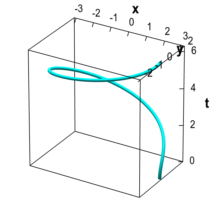
Graph of a function that parametrizes an ellipse. Graph of the vector-valued function $\adllp(t)=(3\cos \frac{t^2}{2\pi})\vc{i} + (2 \sin \frac{t^2}{2\pi}) \vc{j}$. This function parametrizes an ellipse. Its graph, however, is the set of points $(t,3\cos \frac{t^2}{2\pi},2 \sin \frac{t^2}{2\pi})$, which forms a curve that spirals more quickly with increasing $t$.
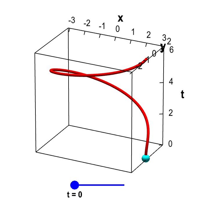
Three-dimensional vector-valued functions can parametrize curves embedded in three-dimensions. The function $\sadllp(t) = (3\cos t)\vc{i} + (2 \sin t) \vc{j} + t\vc{k}$ parametrizes a helix, as shown below. This helix looks like the graph of $\dllp$, above. But, in this case, we have a mapping from the interval $[0,2\pi]$ onto the helix, so this is a parametrized helix. If we wanted to graph $\sadllp$, we would need four dimensions.
Applet loading
Parametrized elliptical helix. The vector-valued function $\sadllp(t)=(3\cos \frac{t^2}{2\pi})\vc{i} + (2 \sin \frac{t^2}{2\pi}) \vc{j}+ t \vc{k}$ parametrizes an elliptical helix, shown in red. This helix is the image of the interval $[0,2\pi]$ (represented by the blue slider) under the mapping of $\sadllp$. For each value of $t$, the cyan point represents the vector $\sadllp(t)$. As you change $t$ by moving the blue point along the interval $[0,2\pi]$, the cyan point traces out the helix.
A special case of a parametrized curve is a parametrized line. In this page, we introduce a simple parametrization of a line. But after seeing how we could change the vector-valued function and still parametrize the same curve, can you think of other types of vector-valued functions that would parametrize a line?
The derivative of a parametrized curve also has special meaning.
Thread navigation
Multivariable calculus
Math 2374
- Previous: Chain rule examples
- Next: Derivatives of parameterized curves
Notation systems
Similar pages
- Derivatives of parameterized curves
- Tangent lines to parametrized curves
- Tangent line to parametrized curve examples
- Parametrized curve and derivative as location and velocity
- Line integrals are independent of parametrization
- Parametrization of a line
- Parametrization of a line examples
- Level sets
- Level set examples
- Translation, rescaling, and reflection
- More similar pages