Introduction to local extrema of functions of two variables
Review of functions of one variable
You remember how to find local extrema (maxima or minima) of a single variable function $f(x)$. Let's assume $f(x)$ is differentiable. Then the first step is to find the critical points $x=a$, where $f\,'(a)=0$. Just because $f\,'(a)=0$, it does not mean that $f(x)$ has a local maximum or minimum at $x=a$. But, at all extrema, the derivative will be zero, so we know that the extrema must occur at critical points.
For example, in the graph below, $f(x)$ is plotted by a green line. The three critical points are marked by colored circles. The red circle marks a local maximum and the blue circle marks a local minimum. The yellow circle marks a critical point that is neither a maximum or a minimum. Even though $f\,'(x)=0$ at the yellow circle, the yellow circle does not mark a local extremum.
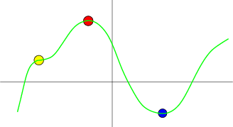
At each of these critical points, the linear approximation (i.e., tangent line) to $f(x)$ is a horizontal line since $f'(a)=0$. We can determine if $f$ has a local extremum at $x=a$ by looking at the secord-order Taylor polynomial, which for a function of one variable is \begin{align*} f(x) \approx f(a) + \frac{1}{2} f\,''(a)(x-a)^2, \end{align*} since $f\,'(a)=0$. As long as $f\,''(a) \ne 0$, the Taylor polynomial says that $f(x)$ looks like the top or bottom of a parabola for $x$ near $a$. If $f\,''(a)>0$, then $f(x)$ is approximately a parabola pointing upward and $f$ has a local minimum at $x=a$, as illustrated by the blue circle, above. If $f\,''(a) < 0$, then $f(x)$ is approximately a parabola pointing downward and $f$ has a local maximum at $x=a$, as illustrated by the red circle, above. On the other hand, if $f\,''(a) = 0$, then the second-order Taylor polynomial doesn't gives us any more information. At the point $x=a$, $f$ could have a local maximum, or it could have a local minimum, or it might not even have a local extremum, as illustrated by the yellow point, above.
Functions of multiple variables
If $f(\vc{x})$ is a function of multiple variables, categorizing local extrema proceeds in an analogous way. So that we can visualize $f(\vc{x})$, we look only at the case of two variables, $\vc{x}=(x,y)$, where we can graph $f(x,y)$ as a surface. Assuming $f(x,y)$ is differentiable, local extrema can occur only at critical points $(x,y) = (a,b)$, where the derivative of $f(x,y)$ is zero, i.e., those points $(a,b)$ where $Df(a,b) = [0 \ 0]$.
If $Df(a,b) = [0 \ 0]$, then the linear approximation (i.e, tangent plane) of $f(x,y)$ at $(a,b)$ is a horizontal plane. As in the one-variable case, we can determine if $f$ has a local extremum at $(a,b)$ by looking at the secord-order Taylor polynomial. If we let $(a,b)=\vc{a}$ (remember that $(x,y)=\vc{x}$), then the second-order Taylor polynomial is \begin{align*} f(\vc{x}) \approx f(\vc{a}) + \frac{1}{2} (\vc{x}-\vc{a})^T Hf(\vc{a}) (\vc{x}-\vc{a}). \end{align*} All this equation says is that, around $\vc{x}=\vc{a}$, the graph of $z=f(x,y)$ looks like a quadric surface (unless $Hf(a,b)$ is zero). In fact, $f(x,y)$ will look like a paraboloid.
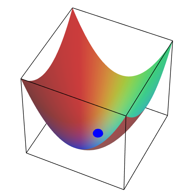
Depending on the second derivative matrix $Hf(a,b)$, the graph of $f(x,y)$ might look like an elliptic paraboloid pointing upward, centered at the point $(a,b)$ (shown by the blue dot, below). In this case, we say that $Hf(a,b)$ is positive definite, and $f$ has a local minimum at $(a,b)$.
Applet loading
A local minimum of a function of two variables. The blue point is a local minimum of a function of two variables.
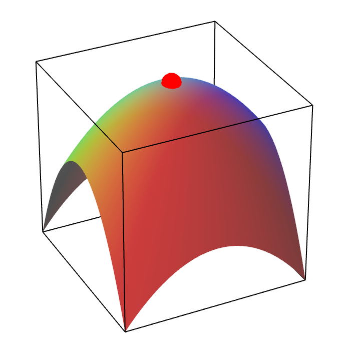
Alternatively, the graph of $f(x,y)$ might look like an elliptic paraboloid pointing downward, centered at the point $(a,b)$ (shown by the red dot, below). In this case, we say that $Hf(a,b)$ is negative definite, and $f$ has a local maximum at $(a,b)$.
Applet loading
A local maximum of a function of two variables. The red point is a local maximum of a function of two variables.
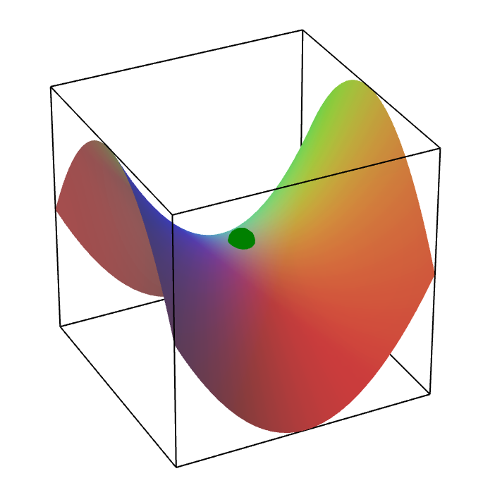
There is a third possibility that couldn't happen in the one-variable case. The graph of $f(x,y)$ might look like a hyperbolic paraboloid centered at the point $(a,b)$ (shown by the green dot, below). In this case, the graph looks like a local maximum if you move in one direction (the direction where one's legs would go if one sat on the saddle) and the graph looks like a local minimum if you move in another direction (the direction corresponding to the front and back if one sat on the saddle). In this case, we say that $Hf(a,b)$ is indefinite, and $f$ has neither a local maximum nor a local minimum at the critical point. Such a critical point is called a saddle point.
Applet loading
A saddle point of a function of two variables. The green point is a saddle point of a function of two variables.
There are other cases, which correspond to the yellow point in the one-variable case, above. These are cases where one cannot tell from the second-order Taylor polynomial if $f$ has a local maximum, a local minimum, or neither at the critical point. One would have to look at higher-order terms of the Taylor polynomial to determine the local behavior of the function.
Here are some examples (which assume knowledge of determining the definiteness of $Hf(a,b)$ that is not discussed in this page.)
Thread navigation
Multivariable calculus
Math 2374
Similar pages
- Two variable local extrema examples
- Local minima and maxima (First Derivative Test)
- Minimization and maximization refresher
- Introduction to Taylor's theorem for multivariable functions
- Solutions to minimization and maximization problems
- Introduction to differentiability in higher dimensions
- Subtleties of differentiability in higher dimensions
- Approximating functions by quadratic polynomials
- Developing an initial model to describe bacteria growth
- Spruce budworm outbreak model
- More similar pages