A model of chemical pollution in a lake
A pristine lake of area 2 km2 and average depth of 10 meters has a river flowing through it at a rate of 10,000 m3 per day. A factory is built beside the river and releases 100 kg of chemical waste into the lake each day. What will be the amounts of chemical waste in the lake on succeeding days?
We develop a discrete dynamical system model as an example of a mathematical model that describes the response of systems to constant infusion of material or energy. We show how these systems can move toward an equilibrium.
Developing the dynamical system model
Deriving a model of chemical pollution in a lake.
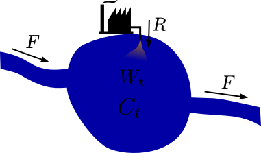
The daily change in chemical waste in the lake is the difference between the amount of chemical released each day by the factory and the amount of chemical that flows out of the lake down the exit river. We will make one key assumption so that we can develop a simple mathematical model: we will assume that upon release from the factory, the chemical quickly mixes throughout the lake so that the chemical concentration in the lake is uniform.
We start by introducing notation. Let $t$ be time measured in days after the factory opens and $W_t$ be the chemical waste in kg in the lake on day $t$. For convenience, we'll also introduce notation for the concentration $C_t$ of chemical waste in kg/m3. Let $V$ be the volume of the lake in m3, $F$ be the daily flow of water through the lake in m3, and $R$ be the daily release of chemicals in kg.
Three of these quantities are constants, and we can view them as parameters of the model. Each of these parameters can be fixed from the data given in the statement of the problem. One parameter is the lake volume, \begin{align*} V &= \mbox{area} \times \mbox{depth} \\ &= 2 \mbox{ km}^2 \times 10 \mbox{ m} \\ &= 2 \times 10^7 \mbox{m}^3. \end{align*} A second parameter is the flow out of the lake in one day, $$F = 10^4 \mbox{ m}^3.$$ The third parameter is the amount of chemical released in a day, $$R = 100 \mbox{ kg}.$$
Given that the volume is fixed, the chemical concentration $C_t$ is just a known multiple of the total chemical waste $W_t$ in the lake. In kg/m, the concentration is $$ C_t = \frac{W_t}{V} = \frac{W_t}{2 \times 10^7}.$$
To derive the dynamical systems model for the waste $W_t$, we look at the change in the amount of chemical on day $t$, which is $$\text{change in chemicals} = W_{t+1} - W_t.$$ The statement of the problem tells us that $R$ (or 100 kg) is the amount of chemical added from the factory each day. If there were no river flowing through the lake, then the simple answer would be that the change $W_{t+1}-W_{t}$ is exactly $R$, and the amount of chemical would steady increase by 100 kg each day.
However, the fact that the river runs through the lake means that some chemicals get removed from the lake and flows downstream. We need to calculate the amount of chemicals (in kg) that is removed from the river each day. We know that the flow of water out the exit river each day is $F$. But that quantity, of course, is water, not chemicals. The amount of chemical waste that leaves the lake each day is equal to the amount of water that leaves the lake that day times the concentration of chemical waste in that water.
To find a formula for flow of chemicals out of the lake, we use that fact we already have an expression for the concentration $C_t$ of chemical in kg/m3. If we multiply this concentration by the daily flow $F$ (in m3), we get an amount $F \times C_t$ in kg of the chemical that is removed from the lake each day. To write our model, we want to express the chemicals solely in terms of $W_t = VC_t$. Replacing $C_t$ with $W_t/V$, we calculate that the amount of chemicals (in kg) removed from the lake per day is $$\frac{FW_t}{V}.$$
Our dynamical system model giving the daily change in chemicals is in the form: change per day = amount added per day - amount removed per day. Summarizing our above findings, the model is \begin{align} W_{t+1}-W_t = R - \frac{F}{V}W_t. \label{pollution_model_change} \end{align}
As a sanity check, we can verify that the units of each term match up. Both $W_t$ and $R$ are in kg. And since both $F$ and $V$ are in m3, the units of the fraction $F/V$ cancel, and the last term in equation \eqref{pollution_model_change} is also in units of kg.
For the given values of $R=100$ and $$\frac{F}{V} = \frac{10^4}{2 \times 10^7} = 5 \times 10^{-4} = 0.0005,$$ the model is $$W_{t+1}-W_t = 100 - 0.0005 W_t.$$
Day 0 is the the day the factory went into operation, so the initial condition is $W_0 =0.$ We can solve equation \eqref{pollution_model_change} for $W_{t+1}$, writing the dynamical system as \begin{align} W_0 &=0\notag\\ W_{t+1} &= R+\left(1- \frac{F}{V}\right)W_t. \label{pollution_model} \end{align} Or, for the given parameter values, the system is \begin{align*} W_0 &=0\notag\\ W_{t+1} &= 100+0.9995W_t. \end{align*}
Solving the dynamical system model
Solving a model of chemical pollution in a lake.
We can compute the amounts of chemical waste in the lake on the first few days. For example, if you put $f(x)=100+0.9995 x$ and $x_0=0$ in the function iteration applet, you'll find that chemical waste after the each of the first four days is 100, 199.95, 299.85, and 399.70 kg. To find out the chemical level at the end of the first year, you'd need to iterate 365 times, which would get tiresome.
The equilibrium state
Before trying to completely solve the model \eqref{pollution_model} for the waste $W_t$ at any day $t$, we can start by asking what happens to the waste level after a long time. For example, the environmentalists may want to know the “eventual state” of the chemical waste in the lake. They would predict that the chemical in the lake will increase until there is no perceptual change on successive days. If this happens, then the state of the system (i.e., $W_t$) is heading toward an equilibrium.
At an equilibrium state, the state variables don't change. In our model, an equilibrium $E$ is a value such that if $W_t = E$, then $W_{t+1}$ is also $E$. We can solve for possible values of $E$ by plugging in $W_t=E$ and $W_{t+1}=E$ into the equation \eqref{pollution_model}. This means that $E$ must satisfy the equation \begin{align} E &= R+\left(1- \frac{F}{V}\right)E. \label{equation_for_E} \end{align} Remember that the parameters $R$, $F$, and $V$ are known numbers, so equation \eqref{equation_for_E} is a single equation for a single unknown $E$, which we can solve for $E$. If we put in values for the statement of the problem, the equation for $E$ is $E=100+0.9995E$ so that $$E = \frac{100}{1 - 0.9995} = 200000.$$ In general, we solve equation \eqref{equation_for_E} as \begin{align*} E &= R+\left(1- \frac{F}{V}\right)E\\ E - \left(1- \frac{F}{V}\right)E &= R\\ \frac{F}{V}E &= R\\ E &= \frac{RV}{F}. \end{align*}
Since for the given parameter values, $E=RV/F = 200,000$, we can conclude that when the chemical in the lake reaches 200,000 kg, the amount that flows out of the lake each day will equal the amount introduced from the factory each day.
The formula $E=RV/F$ makes sense. If we double the chemical release $R$ or the lake volume, then the equilibrium value of the waste doubles. On the other hand, if we double the daily flow, then the equilibrium value of the waste is cut in half.
Deviation from equilibrium
The equilibrium value by itself doesn't tell us anything about the dynamics of the system away from the equilibrium. From the value of $E$ alone, we don't know how quickly the state of system $W_t$ moves toward equilibrium or even if it moves toward equilibrium at all. We need to do some more work to determine the dynamics.
The fact that we know the equilibrium $E$, however, does let us write the dynamical system model more simply. It turns out the equation will be simpler if we write an equation for the difference between the waste level $W_t$ at day $t$ and the equilibrium waste level $E$. Let's define a new variable for this deviation: $$D_t=W_t-E.$$
To calculate an equation for $D_t$, we combine model \eqref{pollution_model} for $W_t$ with equation \eqref{equation_for_E} for $E$: \begin{align*} W_{t+1} &= R+\left(1- \frac{F}{V}\right)W_t\\ E &= R+\left(1- \frac{F}{V}\right)E. \end{align*} By subtracting these equations, we obtain $$W_{t+1} - E = \left(1- \frac{F}{V}\right) (W_t - E).$$ The important consequences are that $R$ disappears and that the equation depends only on $W_t$ and $E$ through their difference $D_t$. We can rewrite it as an equation for $D_t$: \begin{align} D_{t+1} &= \left(1- \frac{F}{V}\right) D_t,\notag\\ D_0 &= -E. \label{equation_for_D} \end{align} The initial condition $D_0=-E$ follows from the fact that $D_0=W_0-E$ and the initial condition for $W_t$ is $W_0=0$.
We've reduced the problem to an equation \eqref{equation_for_D} for $D_t$ that is same form as the initial model for bacteria growth. The equation is another example of exponential growth or decay since the right hand side of the $D_{t+1}$ equation in \eqref{equation_for_D} is linear in $D_t$. In fact, equation \eqref{equation_for_D} can be written as \begin{align*} D_{t+1}&=rD_t\\ D_0 &= -E. \end{align*} with $r=1-F/V$, which is equation (1) from the solving linear systems page with constant $r$. Its solution is \begin{gather} D_t = -E \times r^t, \label{exponential_decay_solution} \end{gather} or $$D_t = -E \left(1- \frac{F}{V}\right)^t.$$
Since $0 < r = 1- F/V < 1$, the evolution of $D_t$ exhibits exponential decay toward zero. Since $D_t$ is the deviation from equilibrium, the chemical waste $W_t = E + D_t$ approaches the equilibrium value.
For the given parameter values, $$D_t = -200000 \times 0.9995^t$$ and the chemical waste after $t$ days is \begin{align} W_t &= E + D_t\notag\\ &= 200000 - 200000 \times 0.9995^t. \end{align} In general, the solution for the chemical waste is \begin{align} W_t &= E -E \left(1- \frac{F}{V}\right)^t. \end{align}
The graph of $W_t$ is shown in below. You can see how $W_t$ approaches $E$ as time increases.
Model of chemical pollution in a lake. The chemical waste $W_t$ in a lake $t$ days after a factory opens moves toward the equilibrium $E=RV/F.$ The waste level $W_t$ is shown by the red curve and the equilibrium value is shown by the horizontal cyan line. You can adjust the parameters by dragging the green points on the sliders. The rate of decay toward equilibrium is captured by the half-life $T_{1/2}$ and the time $T_{0.02}$ for the waste to get 98% the way to equilibrium (i.e., the time for the deviation from equilibrium to decay to 0.02 its original value). You can zoom in and out with the buttons labeled by arrows.
You can read the chemical level of the lake at the end of one year from the graph (when leaving the parameters at their default values) or compute \[ W_{365} = 200000 - 200000 \times 0.9995^{365} \approx 33,000 \mbox{ kg}. \] 33,000 of the 36,500 kg of chemical released into the lake during the first year are still in the lake at the end of the year. Observe that even after 20 years the lake is not quite to equilibrium.
Rate of decay
With exponential decay, we can quantify how fast the system decays to zero with the half-life. For equation \eqref{exponential_decay_solution}, the half-life is (see equation (3) of the half-life page) \begin{gather*} T_{\text{half}}= \frac{\log \frac{1}{2}}{\log r}. \end{gather*} For the given parameters, $r=0.9995$ and the half-life is 1386 days. For $W_t$, the half-life becomes the time it takes the system to make it half-way to the equilibrium value.
Half way to the equilibrium isn't very close, so we might be interested in determining how long it takes the system to get closer to equilibrium. For example, if we double the half life, the deviation from equilibrium is cut in half twice, to one-quarter of its original value, and the waste level evolves to $3/4$ of the equilibrium.
If we want to see how long it takes to get quite close to equilibrium, we can calculate how long it takes for the lake to reach 98 percent of the equilibrium value. We can repeat the half-life calculation with a small change by asking for what $t$ is $D_t$ down to 0.02 times its original value. The only difference from the half-life calculation is to replace 1/2 with 0.02, and the answer is \begin{gather*} T_{0.02}= \frac{\log 0.02}{\log r}. \end{gather*}
For the given parameters, the waste gets to 98% of the equilibrium value after \begin{align*} T_{0.02} &= \frac{\log 0.02}{\log 0.9995} \\ &= 7822 \mbox{ days}\\ &= 21.4 \mbox{ years}. \end{align*}
You can build your own models for similar problems in the exercises.
Thread navigation
Elementary dynamical systems
Similar pages
- Exponential growth and decay modeled by discrete dynamical systems
- Doubling time and half-life of exponential growth and decay
- Chemical pollution model exercises
- Chemical pollution model exercises answers
- Determining stability by cobwebbing linear approximations around equilibria
- Equilibria in discrete dynamical systems
- The idea of stability of equilibria for discrete dynamical systems
- More details on solving linear discrete dynamical systems
- A graphical approach to finding equilibria of discrete dynamical systems
- The idea of a dynamical system
- More similar pages