Evidence for additional structure in real networks
The Erdös-Rényi random network1 (ER random network) is a nice, tractable network model that reduces the large dimension of random networks to a small number of parameters.
In the traditional ER random network model, the probability of any edge is $p$. We can easily extend the ER random network model to networks where this probability could vary across the network. But, the network is still quite simple if we generate all edges independently.
However, networks in the real world show structure that is not captured by random networks with independent connections. Such structure is sometimes called “non-random,” but typically the structure identified can still be captured by different types of random networks.
Motif frequency
A motif in a network is a pattern consisting of a small collection of nodes with a certain combinations of edges. In an ER random network, the probability (or frequency) of a given motif is very simple to calculate. Since each edge must independent exist with probability $p$ and not exist with probability $1-p$, one simply needs to count the number of edges and non-edges in the motif. If a motif contains $n_1$ edges and $n_2$ non-edges, then the probability of that motif must be \begin{gather} \Pr(\text{motif with $n_1$ edges and $n_2$ non-edges}) = p^{n_1}(1-p)^{n_2}. \label{ERmotiffreq} \end{gather}
The only subtlety is knowing whether or not the non-edges are included in the definition of a particular motif. Typically motifs are drawn just by showing the edges included in its definition. Sometimes one must read in-between the lines to know whether or not an edge that is not drawn must be absent for the motif to be counted. If a motif doesn't require edges to be absent, then one must set $n_2=0$ in equation \eqref{ERmotiffreq}.
In a real world networks, the frequencies of motifs don't typically follow equation \eqref{ERmotiffreq}. For example, in neuroscience, Song et. al. found that some three neuron motifs appear much more likely than expected by a ER random network.2 Viewing the network as a directed graph, Song et al. examined the sixteen motifs involving three nodes are shown below. These motifs were defined so that edges not drawn must not exist. All motifs were sixth-order connection motifs, in the sense that they all involve the presence or absence of six edges (i.e., $n_1+n_2=6$).
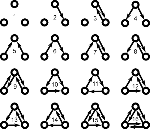
It's difficult to generate large directed graphs where one can specify the frequency of all 16 of these motifs. However, if one is content to specify the frequencies of motifs involving just two edges, then one can generate large graphs with those motif frequencies.
Presence of hubs
Another way in which real world networks differ from ER random networks is in their degree distribution. For simplicity, we restrict this discussion to undirected graphs. If edges are chosen independently, then we expect the degree distribution be to a binomial distribution. This means that most nodes are connected to a similar number of other nodes.
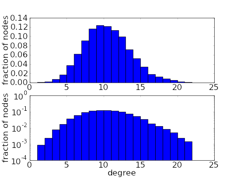
However, one common feature in real world networks is the presence hubs, i.e., nodes with much higher connectivity than the rest. The presencse of hubs gives a long tail in the degree distribution.
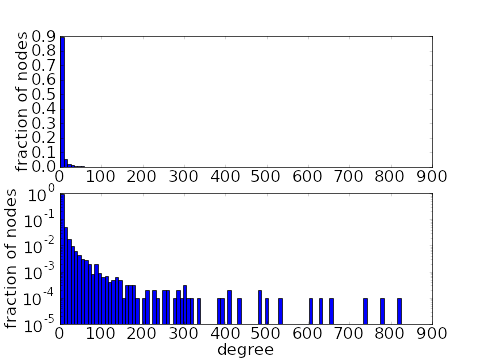
There are a number of network models with long tailed degree distributions. Networks with the thickest tails are the scale-free networks with power-law degree distributions, such as the distribution illustrated above. One can also generate networks with arbitrary degree distributions. It also turns out that one can also generate long-tailed degree distributions by specifying motif frequencies.
Transitivity or clustering
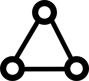
One property of real world networks can be summarized by “your friends are often friends.” Think of a network describing friendship, where nodes are people and a link exists between nodes if the people are friends. Since people commonly socialize in groups larger than two, if you take two friends of a person, its likely that those people are themselves friends. In other words, two nodes that are connected to a third node are more likely to be connected themselves. This property increases the frequency of finding the triangle motif that consist of three mutually connected nodes.
If the edges in a network are generated randomly, then the fact that two nodes have a common neighbor cannot increase the probability that the nodes are connected. For example, in the following Erdös-Rényi random network of 50 nodes and 0.1 connection probability, each node is connected to around 5 other nodes. If you start at a node and follow the connections to two of its neighbors, those neighbors will still have only a small chance (the original 10% connection probability) of being connected.
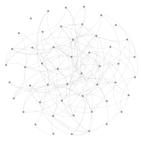
Two related quantities measure the relative frequency of triangles in the graph, or the clustering of the graph: the transitivity $T$ and the clustering coefficient $C$ of a graph. For ER random networks, both $T$ and $C$ are small, while they are comparatively large in most real world networks.
One network model that yields a high clustering coefficient (but still keeps a small mean path length) is the small world network model.
Thread navigation
Network tutorial
- Previous: The absurd high dimensionality of random graphs
- Next: Small world networks
Math 5447, Fall 2020
- Previous: The absurd high dimensionality of random graphs
- Next: Small world networks
Math 5447, Fall 2022
- Previous: The absurd high dimensionality of random graphs
- Next: Small world networks
Similar pages
- Random networks
- The absurd high dimensionality of random graphs
- An introduction to networks
- The degree distribution of a network
- One of the simplest types of networks
- Small world networks
- Scale-free networks
- Generating networks with a desired degree distribution
- Connecting network structure to dynamical properties
- The master stability function approach to determine the synchronizability of a network
- More similar pages