An introduction to networks

Overview of networks

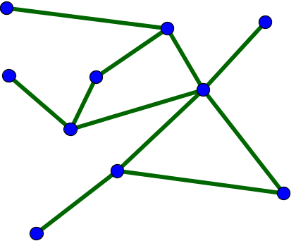
A network is simply a collection of connected objects. We refer to the objects as nodes or vertices, and usually draw them as points. We refer to the connections between the nodes as edges, and usually draw them as lines between points.

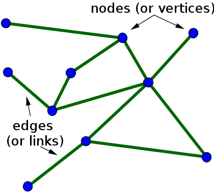
Small undirected network with labeled nodes and edges

In mathematics, networks are often referred to as graphs, and the area of mathematics concerning the study of graphs is called graph theory. Unfortunately, the term graph can also refer to a graph of a function, but we won't use that use of the term when talking about networks. Here, we'll use the terms network and graph interchangeably.

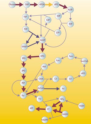
Networks can represent all sorts of systems in the real world. For example, one could describe the Internet as a network where the nodes are computers or other devices and the edges are physical (or wireless, even) connections between the devices. The World Wide Web is a huge network where the pages are nodes and links are the edges. Other examples include social networks of acquaintances or other types of interactions, networks of publications linked by citations, transportation networks, metabolic networks, and communication networks. You can click on the following images for more information about their respective networks.

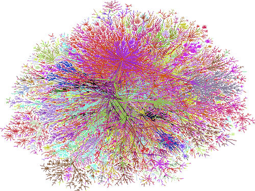
Network of connections between devices within the Internet. Courtesy of Steve Jurvetson. Used under a Creative Commons license.

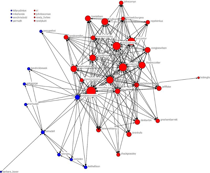
Network of US Congress twitterers showing citation frequency

Network of US congress twitterers. Courtesy of Porter Novelli Global. Used under a Creative Commons license.

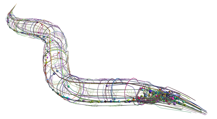
C. elegans connectome merged onto a three-dimensional cellular anatomy model. Courtesy of the OpenWorm project. Used under a MIT License.

Metabolic network model for Escherichia coli. Obtained from Wikimedia Commons.

Types of networks

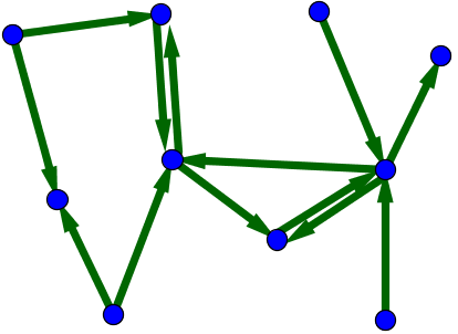
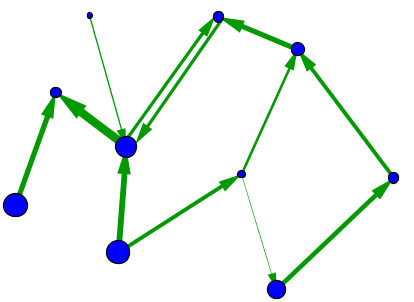
When one tries to model systems such as those mentioned above, one quickly realizes that the simple network model with identical nodes and edges cannot describe important features of real networks. One problem is the edges in this simplest network model are undirected. However, in the World Wide Web, for example, the links between pages are directed. Unfortunately, just because I link from this page to Wikipedia's main page doesn't mean that Wikipedia will put a link from their main page back to this page. Because the edges directed in this way, we need to use a directed network to describe the World Wide Web. In such a directed graph (or digraph, for short), we typically draw the edges as arrows to indicate the direction, as illustrated below.

An undirected network.

A directed network.

Small undirected network with different node and edges types

An undirected network where the nodes and edges have different types, as indicated by their colors and line styles.

Small directed network with weighted nodes and edges

A directed network where the edges and nodes have different weights, as indicated by their sizes.

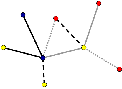
In some networks, not all nodes and edges are created equal. For example, in metabolic networks, nodes may indicate different enzymes which have a wide variety of behaviors, and edges may indicate vastly different types of interactions. To model such difference, one can introduce different types of nodes and edges in the network, as illustrated by the different colors and edge styles, above. In networks where the differences among nodes and edges can be captured by a single number that, for example, indicates the strength of the interaction, a good model may be a weighted graph. One can represent a weighted graph by different sizes of nodes and edges.

In some contexts, one may work with graphs that have multiple edges between the same pair of nodes. One might also allow a node to have a self-connection, meaning an edge from itself to itself. An example of such a network is shown, below.

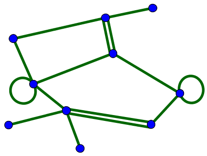
Small undirected network with multiple edges and self-connections

For simplicity, we will focus primarily on unweighted graphs with a single type of node and a single type of edge. We will consider both directed and undirected graphs, but won't allow multiple connections or self-connections.

The adjacency matrix

For unweighted networks of $N$ nodes without multiple connections, the network structure can be represented an $N \times N$ adjacency matrix $A$. Unfortunately, if the network is directed, there exist opposite conventions for how to define the adjacency matrix. In these pages, we will act like mathematicians and define the adjacency matrix so that the component $a_{ij}$ indicates a connection from node $j$ and to node $i$. In this convention, one must read the indices from right to left to determine the direction of the interaction. (Many people use the opposite convention where one must read the indices from left to right.) The adjacency matrix is a matrix of ones and zeros where a one indicates the presence of a connection. Therefore we define $A$ by \begin{gather*} a_{ij} \nobreak{=} \begin{cases} 1 & \text{if there is an edge from node $j$ to node $i$}\\ 0 & \text{otherwise.} \end{cases} \end{gather*}

For example, we could number the vertices of the above directed graph from 1 to 10. In the below figure, we label each edge with the corresponding component of the adjacency matrix.

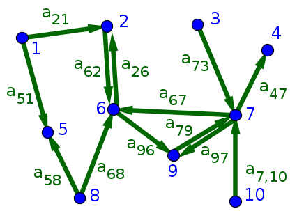
Small directed network with numbered nodes and labeled edges

From the figure, we see that the adjacency matrix has 13 ones corresponding to the 13 edges. Of course, the adjacency matrix contains all 100 entries, the rest of which are zero. \begin{gather*} A \nobreak{=}\left[ \begin{array}{cccccccccc} 0 & 0 & 0 & 0 & 0 & 0 & 0 & 0 & 0 & 0\\ 1 & 0 & 0 & 0 & 0 & 1 & 0 & 0 & 0 & 0\\ 0 & 0 & 0 & 0 & 0 & 0 & 0 & 0 & 0 & 0\\ 0 & 0 & 0 & 0 & 0 & 0 & 1 & 0 & 0 & 0\\ 1 & 0 & 0 & 0 & 0 & 0 & 0 & 1 & 0 & 0\\ 0 & 1 & 0 & 0 & 0 & 0 & 1 & 1 & 0 & 0\\ 0 & 0 & 1 & 0 & 0 & 0 & 0 & 0 & 1 & 1\\ 0 & 0 & 0 & 0 & 0 & 0 & 0 & 0 & 0 & 0\\ 0 & 0 & 0 & 0 & 0 & 1 & 1 & 0 & 0 & 0\\ 0 & 0 & 0 & 0 & 0 & 0 & 0 & 0 & 0 & 0 \end{array} \right] \end{gather*}

Given our convention for the adjacency matrix, you can read all the connections onto a node $i$ by looking across the $i$th row. You can read all the connections from a node $j$ by looking across the $j$th column.

For undirected graphs, the convention for denoting the adjacency matrix doesn't matter, as all edges are bidirectional. In this The bidirectionality means that the adjacency matrix is symmetric.

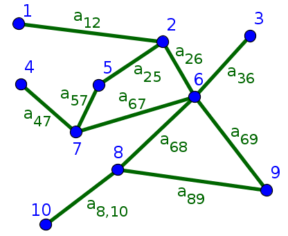
Small undirected network with numbered nodes and labeled edges

For undirected graph represented in the above figure, the eleven edges lead to 22 ones in the adjacency matrix since, by symmetry, each edge leads to two entries in the matrix. For example, the edge between nodes 1 and 2 leads to $a_{12}=1$ and $a_{21}=1$, though we've labeled it by just $a_{12}$ in the above figure. The symmetry of $A$ means that the rows are equal to the columns.

\begin{gather*} A \nobreak{=}\left[ \begin{array}{cccccccccc} 0 & 1 & 0 & 0 & 0 & 0 & 0 & 0 & 0 & 0\\ 1 & 0 & 0 & 0 & 1 & 1 & 0 & 0 & 0 & 0\\ 0 & 0 & 0 & 0 & 0 & 1 & 0 & 0 & 0 & 0\\ 0 & 0 & 0 & 0 & 0 & 0 & 1 & 0 & 0 & 0\\ 0 & 1 & 0 & 0 & 0 & 0 & 1 & 0 & 0 & 0\\ 0 & 1 & 1 & 0 & 0 & 0 & 1 & 1 & 1 & 0\\ 0 & 0 & 0 & 1 & 1 & 1 & 0 & 0 & 0 & 0\\ 0 & 0 & 0 & 0 & 0 & 1 & 0 & 0 & 1 & 1\\ 0 & 0 & 0 & 0 & 0 & 1 & 0 & 1 & 0 & 0\\ 0 & 0 & 0 & 0 & 0 & 0 & 0 & 1 & 0 & 0 \end{array} \right] \end{gather*}

Thread navigation

Math Insight