An introduction to parametrized surfaces
Parametrized surfaces extend the idea of
parametrized curves
to vector-valued functions of two variables.
We can parametrize a curve with a function of one variable.
The function $\dllp: [a,b] \to \R^3$ (confused?) maps the interval $[a,b]$ onto a curve in three dimensions.
For example, $\dllp(t) = (\cos t, \sin t, t)$
parametrizes a helix or
slinky. The below applet shows a helix with one loop,
as we let $t$ range in $[0,2\pi]$.
Parametrized helix. The vector-valued function $\dllp(t)=(\cos t, \sin t, t)$ parametrizes a helix, shown in blue. This helix is the image of the interval $[0,2\pi]$ (shown in cyan) under the mapping of $\dllp$. For each value of $t$, the red point represents the vector $\dllp(t)$. As you change $t$ by moving the cyan point along the interval $[0,2\pi]$, the red point traces out the helix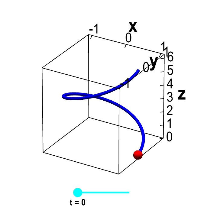
Applet loading
We can parametrize surfaces in the same way. To parametrize surfaces, we simply need a function of two variables. To illustrate the properties of parametrized surfaces, we will use the example function \begin{align*} \dlsp(\spfv,\spsv) = (\spfv\cos \spsv, \spfv\sin \spsv, \spsv). \end{align*} If we fix $\spfv=1$, then $\dlsp(1,\spsv)$ parametrizes the helix as before. If we change $\spfv$ to 0.5, then $\dlsp(0.5,\spsv)$ also parametrizes a helix, but this time with radius 0.5 rather than radius 1.
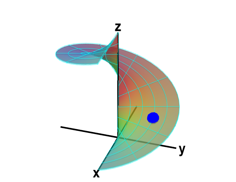
If we let $\spfv$ range from 0 to 1, and let $\spsv$ range from 0 to $2\pi$, then $\dlsp(\spfv,\spsv)$ traces out a whole family of helices, with radii between 0 and 1. The result is a surface called a helicoid, as shown below.

Applet loading
A parametrized helicoid. The function $\dlsp(\spfv,\spsv) = (\spfv\cos \spsv, \spfv\sin \spsv, \spsv)$ parametrizes a helicoid when $0 \le \spfv \le 1$ and $0 \le \spsv \le 2\pi$. You can drag the cyan and magenta points on the sliders to change the values of $\spfv$ and $\spsv$. Or, you can drag the blue point on the helix directly, which will then change $\spfv$ and $\spsv$ so that the blue point is at $\dlsp(\spfv,\spsv)$. If you leave $\spfv$ fixed and change only $\spsv$, then the blue point traces out a helix with radius given by $\spfv$. If you keep $\spsv$ constant and change only $\spfv$, the blue point traces out a straight line.
If we let $\dlr$ be the region where $0 \le \spfv \le 1$ and $0 \le \spsv \le 2\pi$, i.e., $\dlr = [0,1] \times [0, 2\pi]$, then the function $\dlsp$ maps the region $\dlr$ onto the helicoid shown above. We sometimes write this as $\dlsp: \dlr \to \R^3$. (Note the region $\dlr$ is actually a subset of $\R^2$, so we could also say that $\dlsp: \R^2 \to \R^3$.)
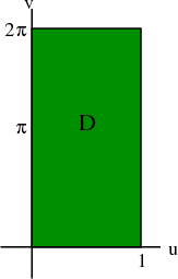
The region $\dlr$ is a rectangle in $\spfv\spsv$-space. Any point $(\spfv,\spsv)$ in $\dlr$ is mapped to the point $\dlsp(\spfv,\spsv)$ on the helicoid. We can demonstrate this map more clearly by replacing the sliders that represent the variables in separate intervals $\spfv \in [0,1]$ and $\spsv \in [0, 2\pi]$ with the rectangle showing that $(\spfv, \spsv) \in [0,1] \times [0, 2\pi]$.
Applet loading
Applet loading
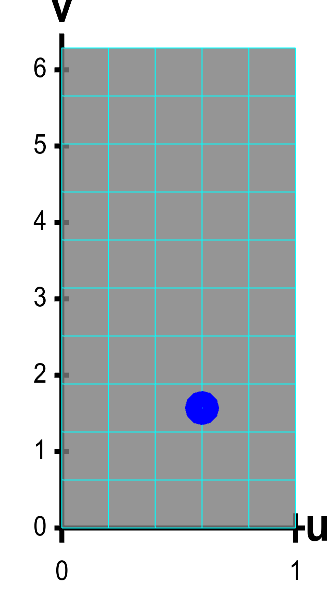
A parametrized helicoid. The function $\dlsp(\spfv,\spsv) = (\spfv\cos \spsv, \spfv\sin \spsv, \spsv)$ parametrizes a helicoid when $(\spfv,\spsv) \in \dlr$, where $\dlr$ is the rectangle $[0,1] \times [0, 2\pi]$. The region $\dlr$, shown as the rectangle in the first panel. You can drag the blue point in $\dlr$ to specify both $\spfv$ and $\spsv$. Alternatively, you can drag the corresponding blue point on the surface in the second panel. In either case, the blue points stay synchronized so that when the blue point in $D$ is at the location $(\spfv, \spsv)$, the blue point on the surface will be at the location $\dlsp(\spfv,\spsv)$.
The region $D$ is divided into small rectangles which are mapped to “curvy rectangles” on the surface. You can click any of the borders of the small rectangles to highlight a curve where one of the variables is constant. Vertical lines in the rectangle $\dlr$ represent curves where $\spfv$ is constant; these correspond to curves that spiral up the helicoid. Horizontal lines in the rectangle $\dlr$ represent curves where $\spsv$ is constant; these correspond to lines that cut across the helicoid. Notice if you drag a blue point along one of these curves, the corresponding blue point in the other panel moves along the corresponding curve. If, for example, you drag the first blue point along the bottom of the rectangle, you change $\spfv$ while leaving $\spsv=0$, and the second blue point moves along the bottom of the helicoid. Similarly, if you drag the blue point along the right side of the rectangle, you change $\spsv$ while leaving $\spfv=1$, and the second blue point spirals around the edge of the helicoid.
In general, the region $\dlr$ does not have to be a rectangle. But in many examples, we let $\dlr$ be a rectangle to make the calculations simpler.
You can see some examples here.
Thread navigation
Multivariable calculus
- Previous: Parametrized curve arc length examples
- Next: Parametrized surface examples
Math 2374
Notation systems
Similar pages
- Surface area of parametrized surfaces
- Orienting surfaces
- Parametrized surface examples
- Calculation of the surface area of a parametrized surface
- Parametrized surface area example
- Normal vector of parametrized surfaces
- A Möbius strip is not orientable
- Parametrization of a line
- Parametrization of a line examples
- An introduction to parametrized curves
- More similar pages