Volume calculation for changing variables in triple integrals
To change variables in a triple integral such as $$\iiint_\dlv f(x,y,z) dV,$$ one uses a mapping of the form $(x,y,z) = \cvarf(\cvarfv,\cvarsv,\cvartv)$. This function maps some region $\dlv^*$ in the $(\cvarfv,\cvarsv,\cvartv)$ coordinates into the original region $\dlv$ of the integral in $(x,y,z)$ coordinates.
In the triple integral change variable story, we illustrate, using the below applet involving an electrode tip, how the change of variable map $\cvarf$ transforms volume as it stretches or compresses different parts of $\dlv^*$ to map it onto $\dlv$.
Applet loading
Applet loading
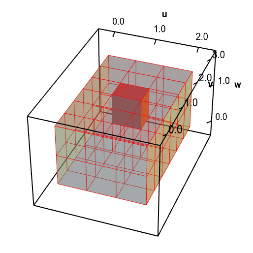
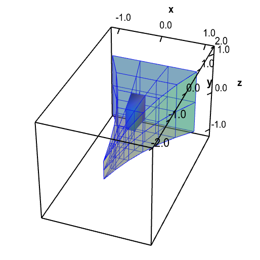
A change of variables for an electrode tip domain changes volume. A change of variables $\cvarf$ maps a rectangular solid $\dlv^*$ (first panel, in red) onto the the electrode tip $\dlv$ (second panel, in blue). It maps each small region of $\dlv^*$ onto a region of a different size in $\dlv$. You can move the highlighted red region in $\dlv^*$ and the highlighted blue region in $\dlv$ by dragging them with your mouse. As you move one region, the corresponding region in the other domain is highlighted. Notice that the red region has a different volume than the corresponding blue region. Especially when the blue region is near the electrode tip, the highlighted blue region is much smaller than the red region.
The original integral is expressed in terms of the volume factor $dV$ which measures volume in the region $\dlv$, i.e., volume in terms of the original variables $x$, $y$, and $z$. In order to change variables and rewrite the integral in terms of the new variables $\cvarfv$, $\cvarsv$, and $\cvartv$, we need to make sure that we are still measuring area in the original region $\dlv$ even though we are going to compute the integral over a new region $\dlv^*$ in the new variables.
To calculate how $\cvarf$ transforms volume, we chop up the region $\dlv^*$ into small boxes of width $\Delta\cvarfv$, depth $\Delta\cvarsv$, and height $\Delta\cvartv$. The following applet illustrates how one of these boxes with lower left corner $(\cvarfv,\cvarsv,\cvartv)$ might be mapped by a change of variables transformation $\cvarf$ into a “curvy region” with one corner being at the point $\cvarf(\cvarfv,\cvarsv,\cvartv)$.

Applet loading
Applet loading
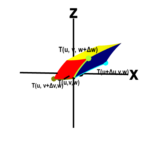
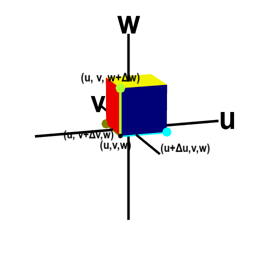
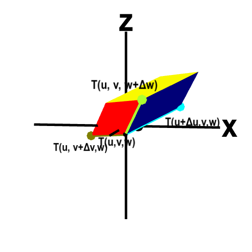
Volume transformation for change of variables in triple integrals. The change of variables function $\cvarf$ transforms a small box (first panel) in $\cvarfv\cvarsv\cvartv$-space to a curvy region (second panel) in $xyz$ space, changing the volume as well as the shape. The original box has one corner at the point $(\cvarfv,\cvarsv,\cvartv)$ and its size is $\Delta\cvarfv \times \Delta\cvarsv \times \Delta\cvarfv$. The corner $(\cvarfv,\cvarsv,\cvartv)$ and the three adjacent corners are labeled. The image of those points under $\cvarf$ form adjacent corners of the curvy region. To help visualize the correspondence between the box and the curvy region under the map $\cvarf$, the edges between the labeled corners are highlighted with different colors.
You can rotate each panel with your mouse to better visual the three dimensional perspective and see all the points. You can drag any of the colored points to change the sizes $\Delta\cvarfv$, $\Delta\cvarsv$, or $\Delta\cvartv$. Dragging the box in the first panel changes the point $(\cvarfv,\cvarsv,\cvartv)$ and hence the shape of the transformation
The volume of the small box in $\cvarfv\cvarsv\cvartv$ space is clearly $\Delta\cvarfv\Delta\cvarsv\Delta\cvartv$, but the volume of the “curvy region” in $xyz$ space is more difficult to calculate. Since the volume of the “curvy region” is the volume of part of the region $\dlv$, it's this volme that we need to calculate the triple integral. Our goal is to calculate an expression for the volume of the “curvy region.” We'll call this volume $\Delta V$ to remind us that this volume is what the $dV$ in the integral represents.
Recall that the triple integral is defined by a Riemann sum where the size of the boxes go to zero. This means we are free to let the dimensions $\Delta\cvarfv$, $\Delta\cvarsv$, and $\Delta\cvartv$ be very small and use any approximation that is valid when they are small. In particular, since we assume that the mapping $\cvarf$ is differentiable, we know that for a small region around the point $(\cvarfv,\cvarsv,\cvartv)$, the function $\cvarf(\cvarfv,\cvarsv,\cvartv)$ is well approximated by its linear approximation centered around the point $(\cvarfv,\cvarsv,\cvartv)$. For small $\Delta\cvarfv$, $\Delta\cvarsv$, and $\Delta\cvartv$, all the points in the small box are close enough to $(\cvarfv,\cvarsv,\cvartv)$ for the linear approximation. As we let the box edges $\Delta\cvarfv$, $\Delta\cvarsv$, and $\Delta\cvartv$ go to zero, any calculation based on the linear approximation will give the correct expression for the volume.
Since linear transformations in three dimensions map parallelepipeds onto parallelepipeds, the “curvy region” must approach a parallelepiped for small $\Delta\cvarfv$, $\Delta\cvarsv$, and $\Delta\cvartv$. If we approximate it as a parallelepiped, we just need to know the location of the vertex $\cvarf(\cvarfv,\cvarsv,\cvartv)$ and the three vertices that share an edge with it. The adjacent vertices $(\cvarfv+\Delta\cvarfv,\cvarsv,\cvartv)$, $(\cvarfv,\cvarsv+\Delta\cvarsv,\cvartv)$, and $(\cvarfv,\cvarsv,\cvartv+\Delta\cvartv)$ on the small box are mapped to the vertices $\cvarf(\cvarfv+\Delta\cvarfv,\cvarsv,\cvartv)$, $\cvarf(\cvarfv,\cvarsv+\Delta\cvarsv,\cvartv)$, and $\cvarf(\cvarfv,\cvarsv,\cvartv+\Delta\cvartv)$, as illustrated above. The resulting parallelepiped with those four vertices is shown below.
Applet loading
Applet loading
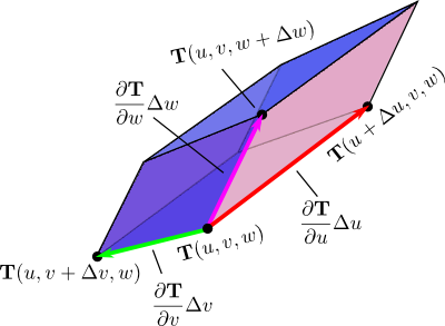
Parallelepiped approximation underlying volume transformation calculation. The change of variables function $\cvarf$ transforms a small box (left) in $\cvarfv\cvarsv\cvartv$-space to a curvy region in $xyz$ space. But, since we view the dimensions $\Delta\cvarfv \times \Delta\cvarsv \times \Delta\cvartv$ as being small, we can approximate the image of the box as the shown parallelepiped (right). Four corners around $(\cvarfv,\cvarsv,\cvartv)$ of the box and the corresponding points on the parallelepiped are labeled (though the dimensions $\Delta\cvarfv, \Delta\cvarsv, \Delta\cvartv$ are replaced by $d\cvarfv, d\cvarsv, d\cvartv$). To help visualize the correspondence between the box and the parallelepiped under the map $\cvarf$, the edges between the labeled corners are highlighted with different colors. Since the image of the box is approximated as a parallelepiped, we can easily calculate its volume using the scalar triple product. Drag the image with your mouse to rotate it and better visualize the mapping.
To calculate the volume of the parallelepiped, we need to take the scalar triple product of the three vectors from the point $\cvarf(\cvarfv,\cvarsv,\cvartv)$ to the neighboring vertices, i.e., the vectors corresponding to the colored edges shown above. These vectors are just the differences between the pair of points, i.e., they are \begin{gather*} \cvarf(\cvarfv+\Delta\cvarfv,\cvarsv,\cvartv)-\cvarf(\cvarfv,\cvarsv,\cvartv),\\ \cvarf(\cvarfv,\cvarsv+\Delta\cvarsv,\cvartv)-\cvarf(\cvarfv,\cvarsv,\cvartv),\\ \cvarf(\cvarfv,\cvarsv,\cvartv+\Delta\cvartv)-\cvarf(\cvarfv,\cvarsv,\cvartv).\\ \end{gather*}
Since we are interested in the limit where $\Delta\cvarfv$, $\Delta\cvarsv$, and $\Delta\cvartv$ go to zero, we can approximate the above differences using the partial derivative limit definition. In this limit, the vectors spanning the parallelepiped edges become \begin{align*} \cvarf(\cvarfv+\Delta\cvarfv,\cvarsv,\cvartv)-\cvarf(\cvarfv,\cvarsv,\cvartv) &= \frac{\cvarf(\cvarfv+\Delta\cvarfv,\cvarsv,\cvartv)-\cvarf(\cvarfv,\cvarsv,\cvartv)}{\Delta\cvarfv} \Delta\cvarfv\\ &\approx \pdiff{\cvarf}{\cvarfv}(\cvarfv,\cvarsv,\cvartv)\Delta\cvarfv\\ \cvarf(\cvarfv,\cvarsv+\Delta\cvarsv,\cvartv)-\cvarf(\cvarfv,\cvarsv,\cvartv) &= \frac{\cvarf(\cvarfv,\cvarsv+\Delta\cvarsv,\cvartv)-\cvarf(\cvarfv,\cvarsv,\cvartv)}{\Delta\cvarsv} \Delta\cvarsv\\ &\approx \pdiff{\cvarf}{\cvarsv}(\cvarfv,\cvarsv,\cvartv)\Delta\cvarsv\\ \cvarf(\cvarfv,\cvarsv,\cvartv+\Delta\cvartv)-\cvarf(\cvarfv,\cvarsv,\cvartv) &= \frac{\cvarf(\cvarfv,\cvarsv,\cvartv+\Delta\cvartv)-\cvarf(\cvarfv,\cvarsv,\cvartv)}{\Delta\cvartv} \Delta\cvartv\\ &\approx \pdiff{\cvarf}{\cvartv}(\cvarfv,\cvarsv,\cvartv)\Delta\cvartv. \end{align*} We label the edges of the parallelepiped, below, with these approximations.
The volume of the curvy region is therefore approximately equal to the absolute value of the scalar triple product of these vectors \begin{align*} \Delta V &\approx \left| \left(\pdiff{\cvarf}{\cvarfv}\Delta\cvarfv \times \pdiff{\cvarf}{\cvarsv}\Delta\cvarsv \right) \cdot \pdiff{\cvarf}{\cvartv}\Delta\cvartv \right|\\ &= \left| \left(\pdiff{\cvarf}{\cvarfv} \times \pdiff{\cvarf}{\cvarsv} \right) \cdot \pdiff{\cvarf}{\cvartv} \right|\Delta\cvarfv\Delta\cvarsv\Delta\cvartv. \end{align*} Given that the derivative matrix of $\cvarf$ is \begin{gather*} \jacm{\cvarf} = \left[\begin{array}{ccc} \pdiff{\cvarfc_1}{\cvarfv} & \pdiff{\cvarfc_1}{\cvarsv} & \pdiff{\cvarfc_1}{\cvartv}\\ \pdiff{\cvarfc_2}{\cvarfv} & \pdiff{\cvarfc_2}{\cvarsv} & \pdiff{\cvarfc_2}{\cvartv}\\ \pdiff{\cvarfc_3}{\cvarfv} & \pdiff{\cvarfc_3}{\cvarsv} & \pdiff{\cvarfc_3}{\cvartv}\\ \end{array} \right], \end{gather*} we can use the determinant notation of the scalar triple product to rewrite our expression for the volume of the curvy region in terms of the determinant of the derivative matrix \begin{gather*} \Delta V \approx \left| \det\jacm{\cvarf}(\cvarfv,\cvarsv,\cvartv)\right|\Delta\cvarfv\Delta\cvarsv\Delta\cvartv. \end{gather*} (This result reflects how the absolute value of the determinant of a linear transformation gives the volume expansion of a linear transformation.)
If we were to form the Riemann sum defining the triple integral in terms of $\cvarfv$, $\cvarsv$, and $\cvartv$, each term in the sum would look like $$f(\cvarf(\cvarfv,\cvarsv,\cvartv)) \left|\det \jacm{\cvarf}(\cvarfv,\cvarsv,\cvartv)\right|\Delta\cvarfv\Delta\cvarsv\Delta\cvartv.$$ Then, letting $\Delta\cvarfv$, $\Delta\cvarsv$, and $\Delta\cvartv$ go to zero, we would obtain the integral \begin{align*} \iiint_\dlv f(x,y,z) \, dV = \iiint_{\dlv^*} f(\cvarf(\cvarfv,\cvarsv,\cvartv)) \left| \det \jacm{\cvarf}(\cvarfv,\cvarsv,\cvartv)\right| \,d\cvarfv\,d\cvarsv\,d\cvartv. \end{align*}
The key point to remember is that that we have to replace the volume factor $dV$ by $\left|\det \jacm{\cvarf}(\cvarfv,\cvarsv,\cvartv)\right|d\cvarfv\,d\cvarsv\,d\cvartv$. You can think of $\left|\det \jacm{\cvarf}(\cvarfv,\cvarsv,\cvartv)\right|$ as the volume expansion factor that captures how the mapping $\cvarf$ is expanding (or compressing) the region $\dlv^*$ at each point as it transforms $\dlv^*$ into $\dlv$.
Thread navigation
Multivariable calculus
- Previous: Introduction to changing variables in triple integrals
- Next: Triple integral change of variable examples
Math 2374
Notation systems
Similar pages
- Introduction to changing variables in triple integrals
- Area calculation for changing variables in double integrals
- Triple integral change of variables story
- Introduction to triple integrals
- Triple integral examples
- Triple integral change of variable examples
- Determinants and linear transformations
- Illustrated example of changing variables in double integrals
- The shadow method for determining triple integral bounds
- The cross section method for determining triple integral bounds
- More similar pages