Area calculation for changing variables in double integrals
To change variables in a double integral such as $$\iint_\dlr f(x,y) dA,$$ one uses a mapping of the form $(x,y) = \cvarf(\cvarfv,\cvarsv)$. This function maps some region $\dlr^*$ in the $(\cvarfv,\cvarsv)$ coordinates into the original region $\dlr$ of the integral in $(x,y)$ coordinates.
As illustrated in the following applet for polar coordinates, the mapping $\cvarf(\cvarfv,\cvarsv)$ transforms area, as it stretches or compresses different parts of $\dlr^*$ to map it into $\dlr$.
Area transformation of polar coordinates map. The transformation from polar coordinates to Cartesian coordinates $(x,y)=\cvarf(r,\theta) = (r \cos\theta, r \sin \theta)$ maps a rectangle $\dlr^*$ in the $(r,\theta)$ plane (left panel) to the region $\dlr$ in the $(x,y)$ plane (right panel). It also maps each small rectangle in $\dlr^*$ to a “curvy rectangle” in $\dlr$. Although the small rectangles in $\dlr^*$ are the same size, the corresponding “curvy rectangles” vary greatly in size. Depending on the coordinates $(r,\theta)$, the map $\cvarf(r,\theta)$ shrinks or expands the area by different amounts. You can visualize the mapping of the small rectangles by dragging the yellow point in either panel; the corresponding small rectangle in $\dlr^*$ and its image in $\dlr$ are highlighted. You can also change the regions $\dlr^*$ and $\dlr$ by dragging the purple and cyan points in either panel.
In the original integral, the relevant area factor $dA$ is in terms of the area in $\dlr$, i.e., in terms of $x$ and $y$. If we wish to change variables and rewrite the integral in terms of $\cvarfv$ and $\cvarsv$, we need to write the area in $\dlr$ in terms of the new variables $\cvarfv$ and $\cvarsv$.
To calculate how $\cvarf$ transforms area, we chop up the region $\dlr^*$ into small rectangles of width $\Delta\cvarfv$ and height $\Delta\cvarsv$. The following figure illustrates how one of these rectangles with lower left corner $(\cvarfv,\cvarsv)$ might be mapped by some map $\cvarf$ into a “curvy rectangle” with one corner being $\cvarf(\cvarfv,\cvarsv)$.
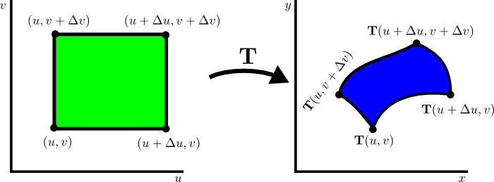
The area of the small rectangle in the $\cvarfv\cvarsv$ plane is clearly $\Delta\cvarfv\Delta\cvarsv$, but the area of the “curvy rectangle” in the $xy$ plane is not so clear. Since the area of the “curvy rectangle” is what counts for the double integral, our goal is to calculate an expression for its area. We'll call this area $\Delta A$ to remind us that the area of the “curvy rectangle” is what the $dA$ in the integral represents.
Since the double integral is defined by a Riemann sum where the size of the rectangles go to zero, we don't need an exact expression for the area of the “curvy rectangle”. We just need an expression that approaches the correct value as the edges of the rectangle $\Delta\cvarfv$ and $\Delta\cvarsv$ go to zero.
When $\Delta\cvarfv$ and $\Delta\cvarsv$ are small, we can approximate the mapping $\cvarf(\cvarfv,\cvarsv)$ with its linear approximation centered around $(\cvarfv,\cvarsv)$. Since linear transformations in two dimensions map parallelograms onto parallelograms, we can conclude that the “curvy rectangle” must approach a parallelogram for small $\Delta\cvarfv$ and $\Delta\cvarsv$.
If we approximate the “curvy rectangle” as a parallelogram, we just need to know the location of three of its vertices. We already know that the vertex $(\cvarfv,\cvarsv)$ on the small rectangle is mapped onto $\cvarf(\cvarfv,\cvarsv)$. The adjacent vertices $(\cvarfv+\Delta\cvarfv,\cvarsv)$ and $(\cvarfv,\cvarsv+\Delta\cvarsv)$ on the small rectangle are mapped to the vertices $\cvarf(\cvarfv+\Delta\cvarfv,\cvarsv)$ and $\cvarf(\cvarfv,\cvarsv+\Delta\cvarsv)$ on the “curvy rectangle”. The vectors from $\cvarf(\cvarfv,\cvarsv)$ to those two points are just the differences of the pairs of points $\cvarf(\cvarfv+\Delta\cvarfv,\cvarsv)-\cvarf(\cvarfv,\cvarsv)$ and $\cvarf(\cvarfv,\cvarsv+\Delta\cvarsv)-\cvarf(\cvarfv,\cvarsv)$. We approximate the “curvy rectangle” as the parallelogram spanned by those two vectors, as illustrated in red in the following figure.
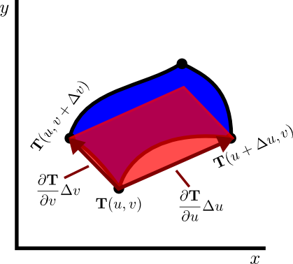
Since we are interested in the limit where $\Delta\cvarfv$ and $\Delta\cvarsv$, and hence $\Delta A$, go to zero, we can make another approximation. Given the limit definition of partial derivatives, we can approximate these vectors in the limit of small $\Delta\cvarfv$ and $\Delta\cvarsv$ as \begin{align*} \cvarf(\cvarfv+\Delta\cvarfv,\cvarsv)-\cvarf(\cvarfv,\cvarsv) &= \frac{\cvarf(\cvarfv+\Delta\cvarfv,\cvarsv)-\cvarf(\cvarfv,\cvarsv)}{\Delta\cvarfv} \Delta\cvarfv\\ &\approx \pdiff{\cvarf}{\cvarfv}(\cvarfv,\cvarsv)\Delta\cvarfv\\ \cvarf(\cvarfv,\cvarsv+\Delta\cvarsv)-\cvarf(\cvarfv,\cvarsv) &= \frac{\cvarf(\cvarfv,\cvarsv+\Delta\cvarsv)-\cvarf(\cvarfv,\cvarsv)}{\Delta\cvarsv} \Delta\cvarsv\\ &\approx \pdiff{\cvarf}{\cvarsv}(\cvarfv,\cvarsv)\Delta\cvarsv. \end{align*} We labeled the edges of the parallelogram, above, with these approximations.
Given this parallelogram approximation, we have a simple way to calculate the approximate area $\Delta A$ of the “curvy rectangle”. The area of the parallelogram is the magnitude of the cross product of the two vectors spanning the parallelogram. Since the vectors $\pdiff{\cvarf}{\cvarfv}(\cvarfv,\cvarsv)\Delta\cvarfv$ and $\pdiff{\cvarf}{\cvarsv}(\cvarfv,\cvarsv)\Delta\cvarsv$ are two-dimensional, we view them as 3D vectors with zero third component so that the cross-product is define. Since they are 2D, we can also represent this area more succinctly by the $2\times 2$ determinant \begin{align*} \Delta A &\approx \left\| \pdiff{\cvarf}{\cvarfv}\Delta\cvarfv \times \pdiff{\cvarf}{\cvarsv}\Delta\cvarsv\right\| = \left\| \pdiff{\cvarf}{\cvarfv} \times \pdiff{\cvarf}{\cvarsv}\right\|\Delta\cvarfv\Delta\cvarsv\\ &=\left|\det \left(\left[ \begin{array}{cc} \pdiff{\cvarfc_1}{\cvarfv} & \pdiff{\cvarfc_2}{\cvarfv}\\ \pdiff{\cvarfc_1}{\cvarsv} & \pdiff{\cvarfc_2}{\cvarsv} \end{array} \right]\right) \right|\Delta\cvarfv\Delta\cvarsv. \end{align*}
We can simplify this expression even further by observing that the above matrix inside the determinant is precisely the derivative matrix $\jacm{\cvarf}$ of the map $\cvarf$. Therefore, the area of the “curvy rectangle” is approximately \begin{align*} \Delta A \approx | \det \jacm{\cvarf}(\cvarfv,\cvarsv)|\Delta\cvarfv\Delta\cvarsv. \end{align*}
If we were to form the Riemann sum defining the integral in terms of $\cvarfv$ and $\cvarsv$, each term in the sum would look like $$f(\cvarf(\cvarfv,\cvarsv)) |\det \jacm{\cvarf}(\cvarfv,\cvarsv)|\Delta\cvarfv\Delta\cvarsv.$$ Then, letting $\Delta\cvarfv$ and $\Delta\cvarsv$ go to zero, we would obtain the integral $$\iint_\dlr f(x,y) dA = \iint_{\dlr^*} f(\cvarf(\cvarfv,\cvarsv)) |\det \jacm{\cvarf}(\cvarfv,\cvarsv)|d\cvarfv\,d\cvarsv.$$
The key point to remember is that that we have to replace the $dA$ by $|\det \jacm{\cvarf}(\cvarfv,\cvarsv)|d\cvarfv\,d\cvarsv$. You can think of $|\det \jacm{\cvarf}(\cvarfv,\cvarsv)|$ as the area expansion factor that captures how the mapping $\cvarf$ is expanding (or compressing) the region $\dlr^*$ at each point as it transforms $\dlr^*$ into $\dlr$.
Thread navigation
Multivariable calculus
- Previous: Introduction to changing variables in double integrals
- Next: Double integral change of variable examples
Math 2374
Similar pages
- Illustrated example of changing variables in double integrals
- Volume calculation for changing variables in triple integrals
- Double integrals as area
- Introduction to changing variables in double integrals
- Double integral change of variable examples
- Triple integral change of variables story
- Determinants and linear transformations
- Introduction to changing variables in triple integrals
- Introduction to double integrals
- Double integrals as iterated integrals
- More similar pages