Illustrated example of changing variables in double integrals

Properties of an example change of variables function

A common change of variables in double integrals involves using the polar coordinate mapping, as illustrated at the beginning of a page of examples. Here we illustrate another change of variables as a further demonstration of how such transformations $(x,y) = \cvarf(\cvarfv,\cvarsv)$ map one region to another. We use the change of variables function \begin{align} (x,y) = \cvarf(\cvarfv,\cvarsv) = (\cvarfv^2-\cvarsv^2, 2\cvarfv\cvarsv). \label{transformation} \end{align}

We first illustrate illustrate the properties of this change of variable function with a series of interactive applets. We then give a concrete problem using the function.

One step of changing variables is determining how the transformation $\cvarf$ maps a region $\dlr^*$ in the $\cvarfv\cvarsv$-plane onto the $xy$-plane. The following applet illustrates this mapping for the case when $\dlr^*$ is a rectangle. You can change the $\dlr^*$ to explore how it is stretched and twisted into an irregularly shaped region $\dlr$.

The Java applet did not load, and the above is only a static image representing one view of the applet. The applet was created with Geogebra. The applet is not loading because it looks like you do not have Java installed. You can click here to get Java.

Nonlinear 2D change of variables map. The map $(x,y)=\cvarf(\cvarfv,\cvarsv) = (\cvarfv^2-\cvarsv^2,2\cvarfv \cvarsv)$ can be used to change variables in a double integral, yielding an integral in $d\cvarfv\,d\cvarsv$ from an integral in $dx\,dy$. To perform such a change of variables, one needs to calculate a region $\dlr^*$ in the $\cvarfv\cvarsv$-plane that is mapped onto the given region $\dlr$ in the $xy$-plane. This applet illustrates how a rectangle $\dlr^*$ in the $\cvarfv\cvarsv$-plane (left panel) is mapped by $\cvarf$ onto a region $\dlr$ in the $xy$-plane (right panel) whose boundaries are parabolas. You can change the regions $\dlr$ and $\dlr^*$ by dragging the purple and cyan points in either panel. To further visualize the action of the map $(x,y)=\cvarf(\cvarfv,\cvarsv)$, you can drag the labeled red and blue points anywhere inside the square $-2 \le \cvarfv \le 2$, $0 \le \cvarsv \le 4$ and the region in the $xy$-plane defined by $y^2/64-16 \le x \le 4-y^2/16$.

Notice how the boundaries of the $\dlr$ are parabolas. For example, the horizontal boundaries (red and green) of the rectangle $\dlr^*$ correspond to lines $\cvarsv=c$ for some constant $c$. Assuming $c \ne 0$, we can solve the second component $(y=2\cvarfv\cvarsv)$ of equation \eqref{transformation} for $\cvarfv$, obtaining $\cvarfv = y/(2c)$. Plugging that result into the first component $(x=\cvarfv^2-\cvarsv^2)$ of equation \eqref{transformation}, we find that $\cvarsv=c$ corresponds to the parabola $x=y^2/(4c^2)-c^2$. When $c$ gets very small, the parabola becomes very steep, as you can notice by, for example, moving the green boundary of $\dlr^*$ close to the $u$-axis. The verticle edges (purple and cyan) of $\dlr^*$ similarly map to parabolic edges of $\dlr$.

Another step in changing variables is determining how the map changes area, i.e., the amount that the map stretches or shrinks $\dlr^*$ as it transforms it into $\dlr$. This stretching is captured by the area expansion factor $| \det \jacm{\cvarf}(\cvarfv,\cvarsv)|$ from equation (1) of the introductory page. For out change of variables function, the matrix of partial derivatives is \begin{align*} \jacm{\cvarf}(\cvarfv,\cvarsv) &= \left(\begin{array}{rr} 2\cvarfv &-2\cvarsv \\ 2\cvarsv & 2\cvarfv \end{array}\right) \end{align*} so that the area expansion factor is \begin{align*} |\det \jacm{\cvarf}(\cvarfv,\cvarsv) | &= |(2\cvarfv)(2\cvarfv) - (-2\cvarsv)(2\cvarsv)| = 4\cvarfv^2 + 4\cvarsv^2. \end{align*} The amount of stretching by $\cvarf$ increases with distance from the origin of the $\cvarfv\cvarsv$-plane.

The following applet allows you to explore how $\cvarf$ is changing area in the irregular region $\dlr$ compared to area in the rectangle $\dlr^*$. See if you can convince yourself that the above formula seems correct.

The Java applet did not load, and the above is only a static image representing one view of the applet. The applet was created with Geogebra. The applet is not loading because it looks like you do not have Java installed. You can click here to get Java.

Area transformation of nonlinear 2D change of variables map. When using the map $(x,y)=\cvarf(\cvarfv,\cvarsv) = (\cvarfv^2-\cvarsv^2,2\cvarfv \cvarsv)$ to change variables in a double integral, one needs to calculate a region $\dlr^*$ in the $\cvarfv\cvarsv$-plane (rectangle in left panel) that is mapped onto the given region $\dlr$ in the $xy$-plane (such as the region in right panel). The transformation $\cvarf$ also maps each small rectangle in $\dlr^*$ to a “curvy rectangle” in $\dlr$. Although the small rectangles in $\dlr^*$ are the same size, the corresponding “curvy rectangles” vary greatly in size. Depending on the coordinates $(\cvarfv,\cvarsv)$, the map $\cvarf(\cvarfv,\cvarsv)$ shrinks or expands the area by different amounts. You can visualize the mapping of the small rectangles by dragging the yellow point in either panel; the corresponding small rectangle in $\dlr^*$ and its image in $\dlr$ are highlighted. You can also change the regions $\dlr^*$ and $\dlr$ by dragging the purple and cyan points in either panel.

To further drive home the concept that $\cvarf$ is taking the rectangle $\dlr^*$ and stretching it into the irregular region $\dlr$, we have one more applet that shows this stretching as an animation. In the right panel, the animation interpolates between $\dlr^*$ and $\dlr$, emphasizing the action of the transformation from $(\cvarfv,\cvarsv)$ coordinates to $(x,y)$ coordinates.

The Java applet did not load, and the above is only a static image representing one view of the applet. The applet was created with Geogebra. The applet is not loading because it looks like you do not have Java installed. You can click here to get Java.

Nonlinear 2D change of variables animation. This animation illustrates the mapping of a rectangle by the change of variables function $(x,y)=\cvarf(\cvarfv,\cvarsv)=(\cvarfv^2-\cvarsv^2,2\cvarfv\cvarsv)$. You can change the function $\cvarf$ by typing in new formulas for its components using the boxes in right panel. The left panel shows a rectangle $\dlr^*$ in the $\cvarfv\cvarsv$-plane, which you can change by dragging the yellow points. The mapping of $\dlr^*$ by $\cvarf$ is illustrated by the animation in the right panel, where the region $\dlr^*$ is stretched into the region $\dlr$, which is the image of $\dlr^*$ under the mapping $\cvarf$. The progress of the animation is shown by the blue slider in the upper left corner. When the blue point moves from left to right, the region in the right panel changes from the reference rectangle $\dlr^*$ into its image $\dlr$. You can stop and start the animation by clicking the button that appears in the lower left of one of the panels. You can also step through the animation by dragging the blue point on the slider. Use the + and - buttons of each panel to zoom in and out.

Since in this applet, the rectangle $\dlr^*$ is not restricted to the upper half-plane $\cvarfv>0$, you can increase the size of $\dlr^*$ so that the mapping of $\cvarf$ is no longer one-to-one. By making $\dlr^*$ be a large portion of any of the half-planes of the $\cvarfv\cvarsv$-plane (such as the half-plane $\cvarfv>0$), you can convince yourself that $\cvarf$ takes any of the half-planes, stretches it around an axis of the $xy$-plane, and maps it to the whole $xy$-plane. If $\dlr^*$ extends beyond one of the half-planes, then it becomes folded, overlaping itself when it is mapped to $\dlr$. This overlapping demonstrates that the mapping is not one-to-one. In this case, $\cvarf$ is not a valid change of variables transformation for $\dlr^*$, and we cannot use equation (1) of the introductory page to calculate the integral. (Note that an overlap only in the final $\dlr$, when the blue slider is all the way to the right, is a problem. The intermediate frames of the animation are artificial and are shown just to guide your eye.)

In the applet, the change of variables is written in component form as $x=\cvarfv^2-\cvarsv^2$ and $y=2\cvarfv\cvarsv$. You can enter different functions of $\cvarfv$ and $\cvarsv$ in the boxes to explore the behavior of different change of variable functions, such as those from the change of variable example page. If you change the function $\cvarf$, then there may be different conditions on $\dlr^*$ to ensure that the map is one-to-one.

A concrete problem with the example function

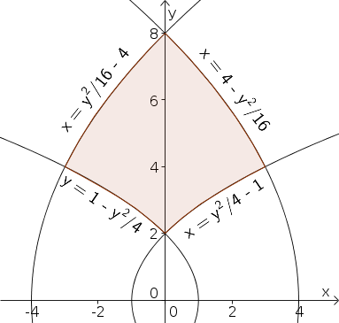
Evaluate the integral $$\iint_\dlr y^2 dA$$ over the region $\dlr$ defined by \begin{gather*} y > 0\\ y^2/16-4 \le x \le y^2/4-1\\ 1-y^2/4 \le x \le 4-y^2/16 \end{gather*} and pictured below. Use the change of variables $x = \cvarfv^2-\cvarsv^2$, $y=2\cvarfv\cvarsv$.

Solution: Initially, it may seem difficult to determine the region $\dlr^*$ that is mapped onto the given region $\dlr$. However, as mentioned above, for the given change of variables, when $\cvarsv=c$ for a constant $c \ne 0$, then $x=y^2/(2c)-c^2$. The two boundaries from the second line are exactly in this form using the constants $c^2=1$ and $c^2=2$. Choosing to use positive $\cvarsv$, the range $y^2/16-4 \le x \le y^2/4-1$ corresponds to the range $1 \le \cvarsv \le 2$.

On the other hand, one can similarly calculate the when $\cvarfv=d$ for constant $d$, this corresponds to $x=d^2-y^2/(4d^2)$. The last two inequalities defining $\dlr$ are in this form for $d^2=1$ and $d^2=4$. Since we require $y>0$ and we have chosen $\cvarsv>0$, we must have $\cvarfv>0$ given that $y=2\cvarfv\cvarsv$. Therefore, we must choose the range $1 \le \cvarfv \le 2$.

It turns out that our change of variables maps the rectangle $\dlr^*$ defined by $1 \le \cvarsv \le 2$ and $1 \le \cvarfv \le 2$ onto the given region $\dlr$. You can use the above applets to convince yourself that this is true.

Since we have already calculated above that the area expansion factor is $4\cvarfv^2+4\cvarsv^2$, the rest is a straightforward integration. Using equation (1) of the introductory page, the integral is \begin{align*} \iint_\dlr y^2 dA &= \int_1^2\int_1^2 (2\cvarfv\cvarsv)^2 (4\cvarfv^2+4\cvarsv^2)d\cvarfv\,d\cvarsv\\ &= \int_1^2\int_1^2 16 (\cvarfv^4\cvarsv^2+ \cvarfv^2\cvarsv^4)d\cvarfv\,d\cvarsv\\ &= \int_1^2 16 \biggl[\frac{1}{5}\cvarfv^5 \cvarsv^2 + \frac{1}{3}\cvarfv^3\cvarsv^4\biggr]_{\cvarfv=1}^{\cvarfv=2} d\cvarsv\\ &= \int_1^2 16 \biggl(\frac{31}{5} \cvarsv^2 + \frac{7}{3}\cvarsv^4\biggr)d\cvarsv\\ &= 16 \biggl[\frac{31}{15} \cvarsv^3 + \frac{7}{15}\cvarsv^5\biggr]_{\cvarsv=1}^{\cvarsv=2}\\ &=\frac{6944}{15}. \end{align*}

More examples

We have more examples to help you master changing variables.