Introduction to the multivariable chain rule
One-variable example
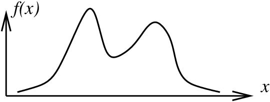
Imagine that the function $f(x)$ gives the height through a mountain range at position $x$. Since this is a one-dimensional example, we are thinking of some cross section through the mountain, as illustrated by this graph of $f(x)$.
Now imagine that you are crossing the mountain range so that your $x$-position at time $t$ is given by $x=g(t)$.
First of all, what is your height at time $t$? It is simply the height of the mountain at the position $x=g(t)$, i.e., $f(x)$ evaluated at $g(t)$, which is $f(g(t))$. We define a function $h(t)$ to give your height at time $t$. It is \begin{align*} h(t) = f(g(t)). \end{align*}
The function $h(t)$ is an example of a composition of functions, meaning it is the result of using function $g$ and then using the function $f$. We often write $h = f \circ g$ or $h(t) = (f \circ g)(t)$.
The chain rule is the rule we use if we want to take the derivative of a composition of functions. In this example, how fast is your height changing as you walk along the path given by $g(t)$? It is simply the derivative of $h$ with respect to $t$: $\displaystyle \diff{h}{t}(t)$. The chain rule gives the derivative of $h$ in terms of the derivatives of $g$ and $f$. You may remember from one-variable calculus that \begin{align} \diff{h}{t}(t) = \diff{f}{x}(g(t))\diff{g}{t}(t). \label{chainrule1D}\tag{1} \end{align} The one-variable chain rule states that the derivative of $h$ is the product of the derivative of $f$ and the derivative of $g$. The only trick to remember is that the derivative of $f$ is evaluated at $g(t)$ (not at $t$). This makes sense since $f$ is a function of position $x$ and $x=g(t)$.
The chain rule makes it a lot easier to compute derivatives. For example, if $g(t)=t^2$ and $f(x)=\sin x$, then $h(t) = \sin (t^2)$. We can easily calculate that \begin{align*} \diff{g}{t}(t) &= g'(t) = 2t,\\ \diff{f}{x}(x) &= f\,'(x)=\cos x,\\ \end{align*} so that \begin{align*} \diff{f}{x}(g(t)) &= f\,'(g(t)) = \cos (t^2). \end{align*} Using the chain rule of equation \eqref{chainrule1D}, we compute that the derivative of $h(t)$ is \begin{align*} \diff{h}{t}(t) = h'(t) = \cos (t^2) (2t). \end{align*} We don't have to separately learn a rule for the derivative of $\sin(t^2)$; we just need to know the derivatives of $\sin x$ and $t^2$.
For more information on the one-variable chain rule, see the idea of the chain rule, the chain rule from the Calculus Refresher, or simple examples of using the chain rule.
The general form of the chain rule
Even though $f$, $g$, and $h$ are one-variable functions, we could use the notation for the derivative of multivariable functions. Remember that the derivative of a multivariable function is its matrix of partial derivatives. We can view the derivatives of $f$, $g$, and $h$ as $1 \times 1$ matrices, \begin{align*} Df(x) &= \left[\diff{f}{x}(x)\right]\\ Dg(t) &= \left[\diff{g}{t}(t)\right]\\ Dh(t) &= \left[\diff{h}{t}(t)\right] \end{align*} Using the notation of matrices of partial derivatives, we can rewrite the one-variable chain rule of equation \eqref{chainrule1D} as \begin{align} Dh(t) = Df(g(t)) Dg(t). \label{chainrule1Dgen}\tag{2} \end{align} Since matrix multiplication of $1 \times 1$ matrices is the same as scalar multiplication, this new equation is just equation \eqref{chainrule1D} in disguised form. Equation \eqref{chainrule1Dgen} is written exactly as the chain rule for higher dimensions. So if you understand what equation \eqref{chainrule1Dgen} means when we use functions $\vc{f}$, $\vc{g}$, and $\vc{h}$ of the form \begin{align*} \vc{f} &: \R^n \to \R^p\\ \vc{g} &: \R^m \to \R^n\notag\\ \vc{h} &: \R^m \to \R^p,\notag \end{align*} (remember function notation) where $\vc{h} = \vc{f} \circ \vc{g}$, then you don't need to read on.
The chain rule in two dimensions
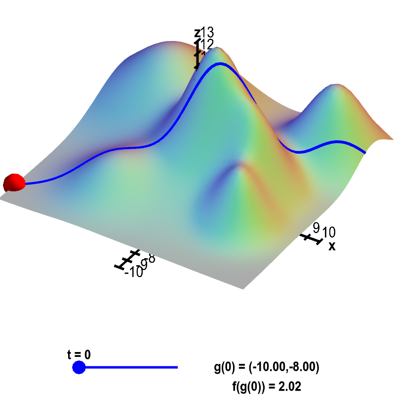
Let's redefine our mountain range function to be a more realistic, two-variable function. Define $f(x,y)$ to be the height of a mountain range at the point $(x,y)$, such as in the graph below. As before, you cross through the mountain range. This time, to specify how you cross the mountain range, you need to specify a path, such as illustrated by the thick blue curve through the mountains below.

Applet loading
Crossing a mountain range. An illustration of a path through a mountain range. The height $f(x,y)$ of a mountain range at position $(x,y)$ is shown by the surface plot. A path through the mountains is shown by the blue curve. The $xy$-coordinates along the path at time $t$ are given by the function $\vc{g}(t)=(g_1(t),g_2(t))$. The blue curve is drawn to be raised at the height the mountain range $f(\vc{g}(t))$ so that it appears to be describing the position of someone walking through the mountain range. For any value of $t$ (changeable via the slider), the $x$ and $y$-coordinates of the red point are $\vc{g}(t)$, and its height is $f(\vc{g}(t))$, as shown in the lower right.
Of course, when you walk through the mountains, you start at one end of the path and, as time progresses, you walk along the path to the other end. You could describe your position during this walk by giving your $x$-position and your $y$-position as functions of time, say $x=g_1(t)$ and $y=g_2(t)$. We could write your position more succinctly if we let $\vc{x}=(x,y)$ and $\vc{g}(t) = (g_1(t),g_2(t))$. Then, your position at time $t$ would be $\vc{x} = \vc{g}(t)$. If you left a trail of (blue) bread crumbs as you walked along the path, the trail would look like the below graph (which, if plotted on top of the mountain, would look like the above blue curve on the mountain).
As before, we are interested in your height as a function of time. (After all, you want to know how much you'll have to climb.) We know that the height of the mountain at position $\vc{x}$ is $f(\vc{x}) = f(x,y)$. We define a function $h(t)$ to give your height at time $t$ as the composition of $f$ and $\vc{g}$: $h(t) = f(\vc{g}(t))$, which we can also write as $h(t) = (f \circ \vc{g})(t)$.
How fast is your height changing as you walk along the path given by the function $\vc{g}(t)$? It is, of course, the derivative of $h(t)$: $\displaystyle \diff{h}{t}$. Since $h$ is a composition of functions, we can use the chain rule to compute its derivative.
Just as in the one-variable case (equation \eqref{chainrule1Dgen}) the chain rule is \begin{align} D{h}(t) = Df(\vc{g}(t)) D{\vc{g}}(t). \label{chainrule2D}\tag{3} \end{align} Again, one important point to remember is that the matrix of partial derivatives of $f$ is evaluated at the point $\vc{x}=\vc{g}(t)$.
We can also write this in terms of components. The matrices of partial derivatives are \begin{align*} Dh(t) &= \left[ \diff{h}{t}(t)\right]\\ Df(\vc{x}) &= \left[ \pdiff{f}{x}(\vc{x}) \,\,\,\, \pdiff{f}{y}(\vc{x})\right]\\ D{\vc{g}}(t) &= \left[ \begin{array}{c} \displaystyle \diff{g_1}{t} (t)\\ \displaystyle \diff{g_2}{t} (t) \end{array} \right]. \end{align*} By multiplying out equation \eqref{chainrule2D}, we find that \begin{align} \diff{h}{t}(t) = \pdiff{f}{x}(\vc{g}(t)) \diff{g_1}{t} (t) + \pdiff{f}{y}(\vc{g}(t))\diff{g_2}{t} (t). \label{chainrule2Dcomp}\tag{4} \end{align} Equation \eqref{chainrule2Dcomp} shows that the chain rule in our two-variable case is just like the one-variable chain rule (equation \eqref{chainrule1D}) applied twice.
The nice thing about equation \eqref{chainrule2D} is that it applies when you take the derivative of any composition of functions. So if you remember equation \eqref{chainrule2D} (and how to multiply matrices), then you'll be all set. You can then even compute the derivative of $\vc{h} = \vc{f} \circ \vc{g}$ for the functions $\vc{f} : \R^n \to \R^p,$ $\vc{g} : \R^m \to \R^n,$ $\vc{h} : \R^m \to \R^p.$ It's just a matter of forming the matrices of partial derivatives and multiplying the matrices. Or, if you prefer, you can look a number of chain rule special cases for particular dimensions $m$, $n$, and $p$, where we multiply out the matrices to obtain chain rule formulas in in terms of their components.
Click here for some chain rule examples.
Thread navigation
Multivariable calculus
- Previous: A differentiable function with discontinuous partial derivatives
- Next: Special cases of the multivariable chain rule
Math 2374
Similar pages
- Multivariable chain rule examples
- Special cases of the multivariable chain rule
- A refresher on the chain rule
- The idea of the chain rule
- Simple examples of using the chain rule
- Introduction to partial derivatives
- Partial derivative examples
- Partial derivative by limit definition
- Introduction to differentiability in higher dimensions
- The multivariable linear approximation
- More similar pages

