Solutions to elementary discrete dynamical systems biology problems
The following is a set of solutions to the elementary discrete dynamical systems biology problems. Let us know if you have a better solution.
Problem 1
- Let $t$ be time in years. Let $m_t =$ the mass of the fish in grams in year $t$. The dynamical system where the fish increases by 100 grams is \begin{align*} m_{t+1}-m_t = 100, \quad \text{for $t=0,1,2, \ldots$} \end{align*}
- Let $m_0=45$ grams, then \begin{align*} m_1 &= m_0+100 = 145 \text{ grams}\\ m_2 &= m_1+100 = 245 \text{ grams}\\ m_3 &= m_2+100 = 345 \text{ grams}\\ m_4 &= m_3+100 = 445 \text{ grams} \end{align*}
- Let $E$ be an equilibrium. Then, $E$ must satisfy \begin{align*} E-E &= 100\\ 0 &= 100 \end{align*} There is no equilibrium (which makes intuitive sense given that the fish is always growing by the same amount).
Problem 2
Let $t$ indicate time in years. Let $e_t$ be the number of elk in the population in the beginning of year $t$. The dynamical system is \begin{align*} \text{population change in a year} &= \text{number born} - \text{number died}. \end{align*}
The change in one year, from the beginning of year $t$ to the beginning of year $t+1$, is just the difference in the population size at the beginning of those two years: $e_{t+1}-e_t$.
The number born in this period is 20% of the population at the beginning of the year, i.e., it is $0.2e_t$.
The number died in this period is one quarter of the population at the beginning of the year, i.e., it is $0.25e_t$.
Putting this all together, we obtain the dynamical system \begin{align*} e_{t+1} - e_t &= 0.2 e_t - 0.25 e_t \end{align*} or \begin{align*} e_{t+1} - e_t &= -0.05 e_t, \quad \text{for $t=0,1,2,3,\ldots$} \end{align*} The dynamical system just captures the fact that there is a net 5% decline in elk population each year.
Let the year $t=0$ correspond to the year when there are 18,000 elk so that $e_0 = 18,000$. To simplify the calculation, let's rewrite the system as \begin{align*} e_{t+1} &=0.95 e_t, \quad \text{for $t=0,1,2,3,\ldots$} \end{align*} where we added $e_t$ to both sides of the equation. Then, we just need to multiply by $0.95$ to calculate the next year's population size. Our result is \begin{align*} e_1 &= 0.95 e_0 = 0.95 \times 18000 = 17,100 \text{ elk}\\ e_2 &= 0.95 e_1 = 0.95 \times 17100 = 16,245 \text{ elk}\\ e_3 &= 0.95 e_2 = 0.95 \times 16245 \approx 15,433 \text{ elk}\\ e_4 &= 0.95 e_3 \approx 0.95 \times 15433 \approx 14,551 \text{ elk} \end{align*}
Let $E$ be an equilibrium of the system. Then, \begin{align*} E - E &= -0.05 E\\ 0 &= -0.05 E\\ E &=0 \end{align*} The only equilibrium is $E=0$, when all the elk in the population have died out.
Problem 3
With 1.1% annual population growth, the population size must be multiplied by $c=1+0.011 = 1.011$ each year. In $t$ years, the population size will be multiplied by $c^t$. The number of years $t$ where $c^t$ is 2 is the doubling time \begin{align*} T_{\text{double}} &= \frac{\log 2}{\log c}\\ &=\frac{\log 2}{\log 1.011}\\ &\approx \frac{0.6931}{0.0109} \approx 63.36 \text{ years.} \end{align*} We used the natural log to calculate the numbers in the fraction, but you would get the same result if you used any other base for the logarithm.
To go from 7 billion to 56 billion people, the population must increase by the factor $56/7 = 8$. The population size must double three times, so the time to 56 billion people is $3 T_{\text{double}} \approx 3 \times 63.36 \approx 190.08$ years.
Problem 4
To capture the 5% annual decrease in the population of Steller sea lions, we need to multiply the population size by $d=1-0.05=0.95$ each year. After $t$ years, we must multiply by $d^t$. The value of $t$ where $d^t$ is one-half is the half-life \begin{align*} T_{\text{half}} &= \frac{\log 1/2}{\log d}\\ &=\frac{\log 1/2}{\log 0.95}\\ &\approx \frac{-0.6931}{-0.05129} \approx 13.51 \text{ years.} \end{align*} We used the natural log to calculate the numbers in the fraction, but you would get the same result if you used any other base for the logarithm.
For the population to go from 40,000 to 10,000, it must decrease by a factor of $40000/10000=4$, or must decrease in half two times. The time for this to occur is two half-lives or $2T_{\text{half}} \approx 2 \times 13.51 \approx 27.03$ years. (Notice that when doing the actual calculation, we didn't round until after multiplying by two. For this reason, the rounded result isn't exactly twice the rounded half-life.)
Problem 5
- Let $t=$ time in days. Let $n_t=$ the number of embryo cells in day $t$. Since the number of cells double each day, the dynamical system to go from day $t$ to day $t+1$ is \begin{align*} n_{t+1} = 2n_t \quad \text{for $t=0,1,2, \ldots$} \end{align*}
- If $t$ is the number of days since fertilization, then the initial condition is $n_0=1$. Since for each day, we multiply the number of cells by 2, the number of cells after $t$ days is \begin{align*} d_t = 2^t. \end{align*}
- A pregnancy of 40 weeks is $40 \cdot 7 = 280$ days long. If the number of cells doubled every day for 280 days, the number of cells after 280 days would be \begin{align*} n_{280} &= 2^{280}\\ &= 1,942,668,892,225,729,070,919,461,906,823,518,906,642,406,839,052,139,521,251,812,409,738,904,285,205,208,498,176\\ &\approx 1.943 \times 10^{84} \end{align*} This number is about 10,000 times larger than the estimated number of atoms in the observable universe. Since a newborn child is typically much smaller than the universe and each cell contains many atoms, we can safely assume that a newborn child has much fewer cells. Therefore, we can conclude that the rate of cell division must slow down during the course of the pregnancy.
Problem 6
Let $t$ denote the number of 5 week periods since some reference time. Let $r_t = $ the number of rabbits in the group in time period $t$. In each time period, the number of rabbits increases by a fixed fraction. We will let that fixed fraction be an unknown parameter, which we'll denote by $f$, where $f=$ the fraction by which the population of rabbits increases in a 5 week period.
With this notation, the change in a five week period is $r_{t+1}-r_t$ and we set this equal to $fr_t$, the fraction $f$ times the population size $r_t$ at the beginning of the period. Our resulting dynamical system model is \begin{align*} r_{t+1}-r_t = fr_t \quad \text{for $t=0,1,2,3, \ldots$} \end{align*}
In the given data, the plot was the population change $r_{t+1}-r_t$ versus the population size $r_t$ at the beginning of the period. Since the data was fit by a line going through the origin with slope 0.3, the line indicates that the population change $r_{t+1}-r_t$ can be modeled as being 0.3 times the population size $r_t$: $r_{t+1}-r_t = 0.3 r_t$. Moreover, if we let $t=0$ denoted the first time period from the data table, then the initial population size is $r_0 = 101$.
We can summarize these results with the dynamical system \begin{align*} r_0 &= 101\\ r_{t+1}-r_t &= 0.3 r_t \quad \text{for $t=0,1,2,3, \ldots$} \end{align*}
As a first step in solving the system, we rewrite it as \begin{align*} r_{t+1} = 1.3r_t \end{align*} by adding $r_t$ to both sides. Since in each time period, the population size is multiplied by 1.3, the solution is \begin{align*} r_t = 1.3^t r_0 = 1.3^t \cdot 101. \end{align*}
Let $T=$ time in weeks, so that $t=T/5$. Plugging that into the solution, the rabbit population at week $T$ is estimated to be \begin{align*} \text{Number of rabbits in week $T$} = 1.3^{T/5}\cdot 101. \end{align*} The model estimates the number of rabbits after 35 weeks to be $$1.3^{35/5}\cdot101=1.3^7 \cdot 101 \approx 634,$$ which is just above the observed number. If the rabbit population continued to grow at the same rate for two years, the number of rabbits would be $$1.3^{104/5}\cdot 101 = 1.3^{20} \cdot 101 \approx 19,195.$$
Problem 7
Let $t=$ time in minutes. Let $b_t=$ the population size of the bacteria in minute $t$. Given that the increase from time $t$ to time $t+1$ is $0.1487$ times the population size at time $t$, the dynamical system model is \begin{align*} b_{t+1}-b_t = 0.1487 b_t, \quad \text{for $t=0,1,2,3 \ldots$} \end{align*}
By adding $b_t$ to both size, we can rewrite the dynamical system as \begin{align*} b_{t+1} = 1.1487 b_t, \quad \text{for $t=0,1,2,3 \ldots$} \end{align*} Given that the population size is multiplied by 1.1487 each time step, the solution is \begin{align*} b_t = 1.1487^t b_0. \end{align*} The population size doubles when $1.1487^t = 2$, i.e., when \begin{align*} t=T_{\text{double}} &= \frac{\log 2}{\log 1.1487}\\ &\approx \frac{0.6931}{0.1386} \approx 5. \end{align*} Therefore, the bacteria population size doubles every 5 minutes. We used the natural log to calculate the numbers in the fraction, but you would get the same result if you used any other base for the logarithm.
If the population continues to grow at this rate for one hour, or sixty minutes, the population increases by the factor $1.1487^{60} \approx 4096$, which is the same as doubling about $60/5=12$ times. In two hours, the population size doubles about 24 times, increasing by a factor of $1.1487^{120} \approx 1.678 \times 10^7$, which is about 16.78 million. In four hours, the population size doubles about 48 times, increasing by a factor of $1.1487^{240} \approx 2.816 \times 10^{14}$, which is about 28.16 trillion.
Let $b_t$ measure the bacteria population size in units of the volume of the beaker, so that $b_t=1$ means the beaker is exactly full. If $t$ is minutes after midnight, then the initial conditions are $b_0=5.959 \times 10^{-8}$. As a double check, we can calculate the population size at 2 AM, when $t=120$. By our solution formula, $$b_{120} = 1.1487^{120} \cdot 5.959 \times 10^{-8} \approx 1.$$ Indeed, the beaker is exactly full at 2 AM.
However, this calculation was just optional, as the problem didn't ask us to calculate that the bacteria completely fill the beaker after two hours. We could have taken that for granted.
Given that the beaker was full at 2 AM, the beaker was half full exactly one doubling time $T_{\text{double}}$ before 2 AM. Since we calculated that $T_{\text{double}}$ was 5 minutes, the beaker was half full at 5 minutes to 2:00, or 1:55 AM.
The bacteria filled one beaker at 2 AM. To fill four beakers, they just need to double two more times. The bacteria fill all four beakers after two doubling times, $2T_{\text{double}}$, or 10 minutes, i.e., at 2:10 AM. Not much time was gained by quadrupling the available space.
Problem 8
Let $t=$ time in years. Let $d_t$ be the deer population size in year $t$. In each year, the population size increases by a factor of $a$, which means the population size is multiplied by $a$ each year. The dynamical system describing this population growth is \begin{align*} d_{t+1} = a d_t, \quad \text{for $t=0,1,2, \ldots$} \end{align*}
Let $E$ be an equilibrium. Then, $E$ must satisfy \begin{align*} E&=aE\\ (1-a)E &=0\\ E &=0 \quad \text{or} \quad a=1. \end{align*} Since the problem stated that $a>1$, we can rule out the second condition and conclude that the only equilibrium is $E=0$.
To determine the stability of the equilibrium, we can solve the dynamical system. The solution is \begin{align*} d_t = a^t d_0. \end{align*} If $d_0=0$, then $d_t=0$ for all time, which we knew must be the case since $E=0$ is an equilibrium. But, if $d_0$ is slightly larger than 0, then $d_t$ will grow with time, given that $a>1$. The solution moves away from the equilibrium $E=0$, so it is unstable.
Each year, the number $b$ must be subtracted off the population size. The modified dynamical system is \begin{align*} d_{t+1} = a d_t - b, \quad \text{for $t=0,1,2, \ldots$} \end{align*} If $E$ is an equilibrium, it must satisfy \begin{align*} E &= aE -b\\ (1-a)E &= -b\\ E &= \frac{-b}{1-a} = \frac{b}{a-1}. \end{align*}
We could divide by $1-a$ since we were given that $a>1$ and new that $1-a \ne 0$. Note that since $a>1$ and $b>0$, both numerator and denominator in the last fraction are positive numbers, and $E>0$.
It turns out that the equilibrium is unstable, but the problem didn't ask you to determine that.
Now, instead of subtracting off the fixed number $b$, we need to subtract off a number proportional to the number of deer at previous time step, i.e., we subtract off $cd_t$. The modified dynamical system is \begin{align*} d_{t+1} = a d_t - cd_t = (a-c)d_t, \quad \text{for $t=0,1,2, \ldots$} \end{align*}
Let $E$ be an equilibrium. It must satisfy \begin{align*} E &= (a-c)E\\ (1-a+c)E &= 0\\ E &=0 \quad \text{or} \quad c=a-1 \end{align*} If the hunting exactly matches the growth rate, i.e., $c= a-1$, then every choice of $E$ is an equilibrium; the population size will never change, as the system becomes $d_{t+1}=d_t$. Moreover, in this case, a solution that starts near an equilibrium does stay near the equilibrium (it doesn't move), so by our definition, we'd have to say all the equilibria are stable when $c=a-1$.
On the other hand, if $c \ne a-1$, then there is only one equilibrium: $E=0$. We can check its stability by solving the equation. In each year, the population is multiplied by $(a-c)$, so after $t$ years, the solution is \begin{align*} d_t = (a-c)^t d_0. \end{align*}
If $c < a-1$, then $a-c > 1$ and the population size grows each year. The hunting is less the natural growth. Now matter how close we make the initial population size to the equilibrium $d_0=0$, it will move away from the equilibrium. The equilibrium is unstable. (Of course, if we started exactly at $d_0=0$, the population would stay at zero, consistent with the fact that $E=0$ is an equilibrium.)
If $a> c > a-1$, then the hunting is greater than the natural growth and the population size decreases each year. In this case, $0 < a-c < 1$, so that $(a-c)^t$ goes to zero with increasing $t$. The solution moves toward the equilibrium, and the equilibrium is stable.
If $c >a$, then we get unphysical results, as the model indicates we hunt more deer than there are. We get a negative population size. We can throw out this case.
Problem 9
The $E$ be an equilibrium. Then, $E=f(E)$ so that \begin{align*} E &= \frac{3E^2}{2+E^2}. \end{align*} We can simplify this equation by multiplying through by $2+E^2$ and getting a cubic equation for $E$. \begin{align*} E(2+E^2) &= 3E^2\\ E^3+2E &= 3E^2\\ E^3-3E^2+2E &=0\\ \end{align*} We can factor out an $E$ and then factor the remaining quadratic expression. \begin{align*} E(E^2-3E+2) &=0\\ E(E-1)(E-2) &=0\\ \end{align*} We end up with the conclusion that $E = 0,1, \text{ or }2$.
On the other hand, the problem just asked to show that 0, 1, and 2 were equilibria, so we could have just plugged those values into any of the versions of the equation for $E$. Since those numbers will satisfy the equation, we could conclude they are equilibria.
The cobwebbing is shown below. The equilibria are represented by the red circles. The cobwebbing shows that if one starts with a value $z_0$ just above or just below the equilibrium $E=1$ the trajectory moves away from the equilibria. The equilibrium $E=1$ is unstable. Moreover, if the initial condition $z_0$ is just larger than 1, the trajectory converges to the equilibrium $E=2$. On the other hand, if the initial condition $z_0$ is just smaller than 1, the trajectory converges to the equilibrium $E=0$.
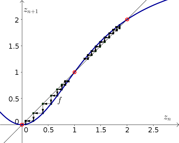
If the banana is shown, the initial condition of $z_0$ around 1.2 will cause the system to evolve to the upper equilibrium of $E=2$. If, on the other hand, a stick is shown, the initial condition of $z_0$ around 0.8 will cause the system to evolve to the lower equilibrium of $E=0$. Since you observe the firing rate has evolved close to the upper equilibrium of $E=2$, the monkey must have been shown a banana.
Thread navigation
Elementary dynamical systems
Similar pages
- The idea of a dynamical system
- An introduction to discrete dynamical systems
- Developing an initial model to describe bacteria growth
- Bacteria growth model exercises
- Bacteria growth model exercise answers
- Exponential growth and decay modeled by discrete dynamical systems
- Discrete exponential growth and decay exercises
- Discrete exponential growth and decay exercise answers
- Doubling time and half-life of exponential growth and decay
- Constructing a mathematical model for penicillin clearance
- More similar pages