Double integral change of variable examples
Example 1
Compute the double integral \begin{align*} \iint_\dlr g(x,y) dA \end{align*} where $g(x,y)=x^2+y^2$ and $\dlr$ is disk of radius 6 centered at origin.
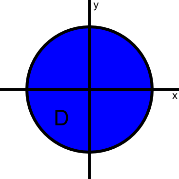
Solution: Since computing this integral in rectangular coordinates is too difficult, we change to polar coordinates. (We chose polar coordinates since the disk is easily described in polar coordinates.) Let \begin{align*} \cvarf(r,\theta) = (r \cos\theta, r \sin \theta). \end{align*} be the change of variables function from polar coordinates into rectangular coordinates.
Then, by the change of variables formula (equation (3) of the introductory page), the integral becomes \begin{align*} \iint_\dlr g(x,y) dA = \iint_{\dlr^{\textstyle *}} g(\cvarf(r,\theta))\left| \det \jacm{\cvarf}(r,\theta)\right| dr\, d\theta, \end{align*} where $\dlr^*$ is the region in the $r\theta$-plane that is mapped by $\cvarf$ onto the disk $\dlr$. In polar coordinates, the disk is described by $0 \le r \le 6$ and $0 \le \theta \le 2\pi$, so the region $\dlr^*$ is a rectangle, making integration simple. See the applet on the polar coordinates map of a rectangle to visualize this transformation from rectangle to disk.
We calculate the pieces of this formula. The integrand $g(x,y)$ becomes \begin{align*} g(\cvarf(r,\theta)) &= g(r\cos \theta, r \sin \theta) \\ &= r^2 \cos^2\theta + r^2 \sin^2 \theta = r^2. \end{align*} The partial derivatives of the transformation $\cvarf(r,\theta)=(r \cos\theta, r \sin \theta)$ are \begin{align*} \pdiff{\cvarfc_1}{r}(r,\theta) & = \pdiff{}{r}(r \cos\theta)= \cos \theta\\ \pdiff{\cvarfc_2}{r}(r,\theta) & = \pdiff{}{r}(r \sin\theta) =\sin \theta\\ \pdiff{\cvarfc_1}{\theta}(r,\theta) & = \pdiff{}{\theta}(r \cos\theta)= -r\sin \theta\\ \pdiff{\cvarfc_2}{\theta}(r,\theta) & = \pdiff{}{\theta}(r \sin\theta) =r \cos \theta. \end{align*} Putting these together, the matrix of partial derivatives of the polar coordinate change of variables is \begin{align*} \jacm{\cvarf}(r,\theta) &= \left( \begin{array}{cc} \cos\theta & -r\sin \theta\\ \sin\theta & r \cos\theta \end{array} \right) \end{align*} which has determinant \begin{align*} \det \jacm{\cvarf}(r,\theta) &= r \cos^2\theta - (-r) \sin^2\theta = r(\cos^2 \theta + \sin^2\theta) = r. \end{align*}
The area expansion factor for the change of variables is $\left|\pdiff{(x,y)}{(r,\theta)}\right|= \left| \det \jacm{\cvarf}(r,\theta)\right| = |r|$. Since we restrict ourselves to $r>0$, we can remove the absolute value and write the area expansion factor as simply $$\left|\pdiff{(x,y)}{(r,\theta)}\right|= \left| \det \jacm{\cvarf}(r,\theta)\right| = r.$$
Now we have all the components to compute the integral. Our final calculation is that \begin{align*} \iint_\dlr g(x,y) dA &= \iint_{\dlr^{\textstyle *}} g(\cvarf(r,\theta))\left| \det \jacm{\cvarf}(r,\theta)\right| dr\, d\theta\\ &=\int_0^{2\pi}\int_0^6 r^2 r\,dr\, d\theta\\ &=\int_0^{2\pi}\frac{r^4}{4}\bigg|_{r=0}^{r=6}d\theta\\ &=\int_0^{2\pi} \frac{6^4}{4} d\theta = \frac{\pi 6^4}{2}. \end{align*}
One nice thing about changing variables to polar coordinates is that you have to compute the area expansion factor only once. For any change of variables to polar coordinates, the area expansion factor will always be $r$. You can simply remember that $dA=dx \,dy = r \, dr\,d\theta$. However, it's important to remember where that $r$ came from, especially if you have to compute any general change of variables, as in the next examples.
In case you have trouble believing that formula, we could motivate the result as follows. Chop up the disk into a grid corresponding to chopping up the $r$ of polar coordinates into intervals of length $\Delta r$ and chopping the $\theta$ of polar coordinates into intervals of length $\Delta \theta$, just as we did for the intro page. A single “curvy rectangle” with a corner $\cvarf(r,\theta)$ is pictured below.
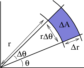
Let $\Delta A$ be area of the “curvy rectangle”. You can see that the area depends on the radius $r$, since its width is approximately $r\Delta \theta$ and its height is approximately $\Delta r$. Hence the area $\Delta A$ is approximately $r \Delta r \Delta \theta$. This sketch captures the reason why $dA$ becomes $r\,dr\,d\theta$ when changing variables to polar coordinates. You can also explore the applet about the area transformation of the polar coordinates mapping to see how the amount of area expansion increases with radius $r$.
Example 2
Evaluate the integral $\iint_D (3x-2y)dA$ over the parallelogram $D$ bounded by the lines $y=\frac{3}{2}x - 4$, $y=\frac{3}{2}x+2$, $y=-2x +1$, and $y=-2x+3$. Use the linear change of variables $$(x,y)=\cvarf(\cvarfv,\cvarsv)=(\cvarfv+2\cvarsv, -2\cvarfv+3\cvarsv).$$
Solution: Since the change of variables is linear, we know know that it maps parallelograms onto parallelograms. If we transform the equations for the parallel lines in terms of the variables $\cvarfv$ and $\cvarsv$, we will again get equations for parallel lines.
Rewrite the equations for the parallelogram boundaries as \begin{align*}3x -2y&=8\\ 3x-2y&=-4\\ 2x+y&=1\\ 2x+y&=3. \end{align*} We can transform the two distinct left hand sides of these equations into $\cvarfv$ and $\cvarsv$ by plugging in $(x,y)=\cvarf(\cvarfv,\cvarsv)$: \begin{align*} 3x-2y &= 3(\cvarfv+2\cvarsv)-2(-2\cvarfv+3\cvarsv)\\ &= 7\cvarfv\\ 2x+y &= 2(\cvarfv+2\cvarsv)+(-2\cvarfv+3\cvarsv)\\ &= 7\cvarsv. \end{align*} Now, the reasons for this choice of change of variables becomes clear. $\cvarf$ maps a rectangle $D^*$ in the $uv$-plane onto the parallelogram $D$. The boundaries of the rectangle $D^*$ are $7\cvarfv = 8$, $7\cvarfv=-4$, $7\cvarsv=1$, and $7\cvarsv=3$. Also, the integrand is simply $7\cvarfv$.
The only remaining point is to calculate the area expansion factor $| \det \jacm{\cvarf}(\cvarfv,\cvarsv)|$. Since, \begin{align*} \jacm{\cvarf}(\cvarfv,\cvarsv) &= \left(\begin{array}{rr} 1 &2 \\ -2 & 3 \end{array}\right), \end{align*} the area expansion factor is $| \det \jacm{\cvarf}(\cvarfv,\cvarsv)| = | (1)(3)-(2)(-2)| = 7$. The integral is \begin{align*} \iint_D (3x-2y)dA &= \int_{1/7}^{3/7} \int_{-4/7}^{8/7}49 \cvarfv \,d\cvarfv\,d\cvarsv\\ &=\int_{1/7}^{3/7} \frac{49}{2} \cvarfv^2 \bigg|_{\cvarfv=-4/7}^{\cvarfv=8/7} d\cvarsv\\ &= \int_{1/7}^{3/7}24 d\cvarsv = \frac{48}{7}. \end{align*}
Example 3
Evaluate \begin{align*} \iint_\dlr \frac{y^2}{x} dx\,dy \end{align*} where $\dlr$ is the region between the parabolas $x=1-y^2$ and $x=3(1-y^2)$. Use the change of variables $(x,y) = \cvarf(\cvarfv,\cvarsv) = (\cvarsv(1-\cvarfv^2), \cvarfv)$.
Solution: We begin by drawing picture of the region $\dlr$, making special note of the corners, or points where the parabolas intersect: $(0,-1)$ and $(0,1)$ .
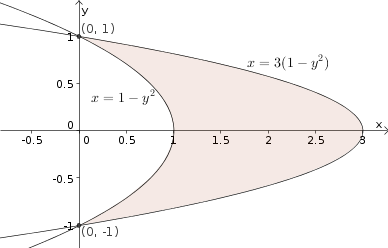
We need to determine the region $\dlr^*$ that $\cvarf$ maps onto $\dlr$. First, observe that, for a fixed $\cvarsv=c$, the curve traced out by $(x,y)=\cvarf(\cvarfv,c)=(c(1-\cvarfv^2),\cvarfv)$ as one varies $\cvarfv$ is the parabola $x=c(1-y^2)$. Moreover, if we let $\cvarfv$ range from $-1$ to $1$, then the curve will go from the point $(0,-1)$ to the point $(0,1)$, just like we need for our region $\dlr$. As long as we keep $\cvarsv$ between 1 and 3, these curves will be inside the region $\dlr$. Therefore, $\dlr$ corresponds to $-1 \le \cvarfv \le 1$ and $1 \le \cvarsv \le 3$. The region $\dlr^*$ that we need for our change of variables is the rectangle $[-1,1] \times [1,3]$ in the $\cvarfv\cvarsv$-plane.
Next, we calculate the area expansion factor. Since \begin{align*} \det\jacm{\cvarf}(\cvarfv,\cvarsv)= \left| \begin{array}{cc} -2\cvarfv\cvarsv & 1-\cvarfv^2\\ 1 & 0 \end{array} \right| = 0 -(1-\cvarfv^2) = \cvarfv^2-1, \end{align*} the area expansion factor is the absolute value \begin{align*} \left|\det\jacm{\cvarf}(\cvarfv,\cvarsv) \right| = |\cvarfv^2-1| = 1-\cvarfv^2. \end{align*} The reason we chose $1-\cvarfv^2$ for the absolute value is that we know that $-1 \le \cvarfv \le 1$ in $\dlr^*$, i.e., $1-\cvarfv^2 \ge 0$. The fact that the area expansion factor goes to zero when $\cvarfv$ goes to $\pm 1$ is consistent with the fact that $\cvarf$ is pinching the region $\dlr$ to the points $(0, \pm 1)$ as $\cvarfv$ approaches $\pm 1$.
Putting it all together, the integral is \begin{align*} \iint_\dlr \frac{y^2}{x} dx\,dy &= \int_1^3 \int_{-1}^1 \frac{\cvarfv^2}{\cvarsv(1-\cvarfv^2)} (1-\cvarfv^2) d\cvarfv\,d\cvarsv\\ &= \int_1^3 \int_{-1}^1 \frac{\cvarfv^2}{\cvarsv} d\cvarfv\,d\cvarsv\\ &= \int_1^3 \frac{\cvarfv^3}{3\cvarsv} \bigg|_{\cvarfv=-1}^{\cvarfv=1}d\cvarsv\\ &= \int_1^3 \frac{2}{3\cvarsv} d\cvarsv\\ &= \frac{2}{3} \log |\cvarsv| \bigg|_1^3 = \frac{2}{3}(\log 3 - \log 1) = \frac{2}{3}\log 3. \end{align*}
Understanding the geometric properties of this change of variables
You can use this applet to visualize how $\cvarf$ is stretches the rectangle $\dlr^*$ onto the given region $\dlr$. Change the transformation in the applet to correspond to the $\cvarf$ of this function. (The transformation $\cvarf$ of this problem in component form is $x=\cvarsv(1-\cvarfv^2)$ and $y=u$, but you'll need to type $\cvarsv * (1-\cvarfv \wedge 2)$ in the box for $x$ in order to have the applet accept the function.) Then, if you change the rectangle to correspond to $\dlr^*$, it should be morphed into the parabolic region $\dlr$. If you are really observant, you may notice that $\cvarf$ flips the region $\dlr^*$ over as it maps it onto $\dlr$; this flipping corresponds to the fact that $\det \jacm{\cvarf}(\cvarfv,\cvarsv)$ is negative. See this page to see more on the relationship between determinants and the geometry of mappings.
Example 4
Evaluate \begin{align*} \iint_\dlr (x^2-y^2)\, dx\,dy \end{align*} where $\dlr$ is the region pictured below.
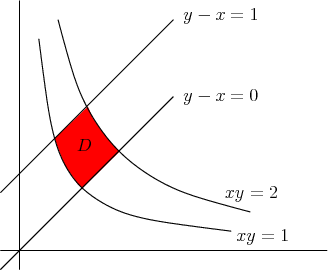
Solution: The region can be described simply if we change to coordinates $\cvarfv$ and $\cvarsv$ where \begin{align} \cvarfv &= y-x\notag\\ \cvarsv&=xy \label{thechangevar} \end{align} With this change of variables, our new region of integration $\dlr^*$ is $0 \le \cvarfv \le 1$, $1 \le \cvarsv \le 2$.
Our change of variables as expressed in equation \eqref{thechangevar} gives $\cvarfv$ and $\cvarsv$ in terms of $x$ and $y$. In our change of variables formula, we need to have $x$ and $y$ expressed in terms of $\cvarfv$ and $\cvarsv$ using some function $(x,y)=\cvarf(\cvarfv,\cvarsv)$. So one way to solve this problem is to solve equation \eqref{thechangevar} for $x$ and $y$ to determine the function $\cvarf$. We could then compute \begin{align*} \pdiff{(x,y)}{(\cvarfv,\cvarsv)} = \det \jacm{\cvarf}(\cvarfv,\cvarsv), \end{align*} which is what we need for the change of variables formula.
For this example, we will use another method that skips this step. We will leave $\cvarfv$ and $\cvarsv$ expressed in terms of $x$ and $y$ (as in equation \eqref{thechangevar}) and compute $\displaystyle \pdiff{(\cvarfv,\cvarsv)}{(x,y)}$ instead of $\displaystyle\pdiff{(x,y)}{(\cvarfv,\cvarsv)}$. Since we know that \begin{align*} \pdiff{(x,y)}{(\cvarfv,\cvarsv)} = \frac{1}{\displaystyle \pdiff{(\cvarfv,\cvarsv)}{(x,y)}}, \end{align*} we can easily get the correct factor for our change of variables formula.
To compute $\displaystyle \pdiff{(\cvarfv,\cvarsv)}{(x,y)}$, we view $\cvarfv$ and $\cvarsv$ as functions of $x$ and $y$: $\cvarfv(x,y)$ and $\cvarsv(x,y)$. The partial derivatives of $\cvarfv$ and $\cvarsv$ with respect to $x$ and $y$ are \begin{align*} \pdiff{\cvarfv}{x} = -1, \qquad \pdiff{\cvarfv}{y} = 1, \qquad \pdiff{\cvarsv}{x} = y, \qquad \text{and} \qquad \pdiff{\cvarsv}{y} = x. \end{align*} We compute \begin{align*} \pdiff{(\cvarfv,\cvarsv)}{(x,y)} &= \det \left( \begin{array}{cc} \displaystyle \pdiff{\cvarfv}{x} & \displaystyle \pdiff{\cvarfv}{y}\\ \displaystyle \pdiff{\cvarsv}{x} & \displaystyle \pdiff{\cvarsv}{y} \end{array} \right)\\ &= \pdiff{\cvarfv}{x} \pdiff{\cvarsv}{y} - \pdiff{\cvarfv}{y}\pdiff{\cvarsv}{x}\\ &= -x -y, \end{align*} so that \begin{align*} \pdiff{(x,y)}{(\cvarfv,\cvarsv)} = \frac{1}{-x -y}. \end{align*} The factor we need for our change of variables formula is then \begin{align*} \left|\pdiff{(x,y)}{(\cvarfv,\cvarsv)}\right| = \frac{1}{x +y} \end{align*} since $x$ and $y$ are positive in our domain.
Once we change variables, we will need to integrate over the region $\dlr^*$ the expression \begin{align*} (x^2 - y^2)\frac{1}{x+y}. \end{align*} Since we can factor $x^2 - y^2 = (x-y)(x+y)$ the above expression simplifies to $x-y$.
Since the integral over $\dlr^*$ is an integral in $\cvarfv$ and $\cvarsv$, we need to write $x-y$ in terms of $\cvarfv$ and $\cvarsv$. Glancing at equation \eqref{thechangevar}, we see that $x-y=-\cvarfv$, so we simply need to integrate $-\cvarfv$ over the region $\dlr^*$.
Our integral is \begin{align*} \int_\dlr (x^2-y^2) dx\, dy &= \left.\iint_{\dlr^{\textstyle *}}\right.-\cvarfv\,d\cvarfv\,d\cvarsv\\ &= -\int_1^2\int_0^1 \cvarfv\,d\cvarfv\,d\cvarsv\\ &= -\int_1^2 \left.\left.\frac{\cvarfv^2}{2}\right|_0^1\right. d\cvarsv\\ &= -\int_1^2 \frac{1}{2} d\cvarsv = -\frac{1}{2} \end{align*} where $x$ and $y$ are functions of $\cvarfv$ and $\cvarsv$.
Example 5
Evaluate \begin{align*} \iint_{\dlr_c} e^{-x^2-y^2} dA \end{align*} where $\dlr_c$ is the region in the first quadrant of the $xy$-plane where $x^2+y^2< c^2$.
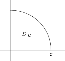
Solution: Change to polar coordinates. Region is sector: $0 \le \theta \le \pi/2$ and $0 \le r \le c$. \begin{align*} \iint_{\dlr_c} e^{-x^2-y^2} dA &= \int_0^{\pi/2} \int_0^c e^{-r^2}r\,dr\,d\theta\\ &= \int_0^{\pi/2} \left.\left.-\frac{1}{2} e^{-r^2}\right|_0^c\right. d\theta\\ &= \frac{1}{2} \left(1-e^{-c^2}\right) \int_0^{2/\pi} d\theta\\ &= \frac{\pi}{4} \left(1-e^{-c^2}\right) \end{align*}
Another example
You can check out another example where the transformation of the change of variables function is illustrated by interactive graphics.
Thread navigation
Multivariable calculus
- Previous: Area calculation for changing variables in double integrals
- Next: Illustrated example of changing variables in double integrals
Math 2374
Similar pages
- Introduction to changing variables in double integrals
- Area calculation for changing variables in double integrals
- Illustrated example of changing variables in double integrals
- Introduction to double integrals
- Double integrals as iterated integrals
- Double integral examples
- Double integrals as volume
- Examples of changing the order of integration in double integrals
- Double integrals as area
- Double integrals where one integration order is easier
- More similar pages