Introduction to changing variables in double integrals
Imagine that you had to compute the double integral \begin{align} \iint_{\dlr} g(x,y) dA \label{integralrect} \end{align} where $g(x,y)=x^2+y^2$ and $\dlr$ is the disk of radius 6 centered at the origin.
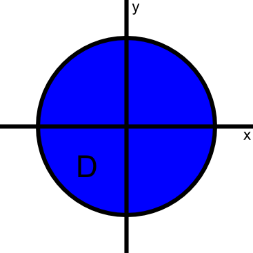
In terms of the standard rectangular (or Cartesian) coordinates $x$ and $y$, the disk is given by \begin{gather*} -6 \le x \le 6\\ -\sqrt{36-x^2} \le y \le \sqrt{36-x^2}. \end{gather*} We could start to calculate the integral in terms of $x$ and $y$ as \begin{align*} \iint_{\dlr} g(x,y) dA = \int_{-6}^6 \int_{-\sqrt{36-x^2}}^{\sqrt{36-x^2}} (x^2+y^2) \, dy \, dx\ = \text{a mess}. \end{align*}
It turns out that this integral would be a lot easier if we could change variables to polar coordinates. In polar coordinates, the disk is the region we'll call $\dlr^*$ defined by $0 \le r \le 6$ and $0 \le \theta \le 2\pi$. Hence the region of integration is simpler to describe using polar coordinates.
Moreover, the integrand $x^2+y^2$ is simple in polar coordinates because $x^2+y^2 = r^2$. Using polar coordinates, our lives will be a lot easier because it seems that all we need to do is integrate $r^2$ over the region $\dlr^*$ defined by $0 \le r \le 6$ and $0 \le \theta \le 2\pi$.
Unfortunately, it's not quite that easy. We need to account for one more consequence of changing variables, which is how changing variables changes area. You may recall that $dA$ stands for the area of a little bit of the region $\dlr$. In rectangular coordinates, we replaced $dA$ by $dx\,dy$ (or $dy\,dx$). We need to determine what $dA$ becomes when we change variables. As you will see, in polar coordinates, $dA$ does not becomes $dr \, d\theta$.
The relationship between rectangular $(x,y)$ and polar $(r,\theta)$ coordinates is given by $x=r\cos \theta$, $y=r\sin\theta$. To see how area gets changed, let's write the change of variables as the function \begin{align} (x,y)=\cvarf(r,\theta) = (r \cos\theta, r \sin \theta). \label{polartrans} \end{align} The function $\cvarf(r,\theta)$ gives rectangular coordinates in terms of polar coordinates. The transformation $\cvarf$ gives the perspective of polar coordinates as a mapping from the polar plane to the Cartesian plane. The below applet shows how $\cvarf$ maps a rectangle $\dlr^*$ in the polar plane into the region $\dlr$ in the Cartesian plane. To make $\dlr^*$ and $\dlr$ correspond to the rectangle and disk of our example, you can expland the rectangle $\dlr^*$ to its maximum size.
Polar coordinates map of rectangle. The transformation from polar coordinates to Cartesian coordinates $(x,y)=\cvarf(r,\theta) = (r \cos\theta, r \sin \theta)$ can be viewed as a map from the polar coordinate $(r,\theta)$ plane (left panel) to the Cartesian coordinate $(x,y)$ plane (right panel). This transformation maps a rectangle $\dlr^*$ in the $(r,\theta)$ plane into a region $\dlr$ in the $(x,y)$ plane that is the part of an angular sector inside an annulus. You can change the regions $\dlr^*$ and $\dlr$ by dragging the purple or cyan points in either panel. To further visualize the action of the map $(x,y)=\cvarf(r,\theta)$, you can drag the labeled red and blue points anywhere inside the large rectangle $0 \le r \le 6$, $0 \le \theta <2\pi$ and corresponding disk $x^2+y^2 \le 6^2$.
Do you understand why the disk looks like a rectangle in polar coordinates (i.e., why the region $\dlr^*$ on the left that maps onto the disk is a rectangle)? Remember, the disk is described by $0 \le r \le 6$ and $0 \le \theta \le 2\pi$, which is a rectangle when plotted in the $r\theta$-plane.
We can say that $\cvarf(r,\theta)$ parametrizes $\dlr$ for $(r,\theta)$ in $\dlr^*$. This uses the same language that we used when parametrizing a curve. We'll use it again when we talk about parametrizing surfaces.
To look at how $\cvarf(r,\theta)$ changes area, we can chop up the region $\dlr^*$ into small rectangles of width $\Delta r$ and height $\Delta \theta$. The function $\cvarf(r,\theta)$ maps each of these small rectangles into a “curvy rectangle” in $\dlr$, as shown below. (As above, you need to expand the rectangle $\dlr^*$ in the left panel to its maximum size to make the $\dlr^*$ and $\dlr$ of the applet correspond to the rectangle and disk of our example.)
Area transformation of polar coordinates map. The transformation from polar coordinates to Cartesian coordinates $(x,y)=\cvarf(r,\theta) = (r \cos\theta, r \sin \theta)$ maps a rectangle $\dlr^*$ in the $(r,\theta)$ plane (left panel) to the region $\dlr$ in the $(x,y)$ plane (right panel). It also maps each small rectangle in $\dlr^*$ to a “curvy rectangle” in $\dlr$. Although the small rectangles in $\dlr^*$ are the same size, the corresponding “curvy rectangles” vary greatly in size. Depending on the coordinates $(r,\theta)$, the map $\cvarf(r,\theta)$ shrinks or expands the area by different amounts. You can visualize the mapping of the small rectangles by dragging the yellow point in either panel; the corresponding small rectangle in $\dlr^*$ and its image in $\dlr$ are highlighted. You can also change the regions $\dlr^*$ and $\dlr$ by dragging the purple and cyan points in either panel.
The area of each small rectangle in $\dlr^*$ is $\Delta r \Delta \theta$. But we don't care about area in $\dlr^*$. The $dA$ in the integral of equation \eqref{integralrect} is based on area in $\dlr$ not area in $\dlr^*$. So we need to estimate the area of each “curvy rectangle” in $\dlr$, which we'll denote by $\Delta A$.
We can calculate the area of the “curvy rectangle” by approximating it as a parallelogram with sides $\pdiff{\cvarf}{r} \Delta r$ and $\pdiff{\cvarf}{\theta}\Delta\theta$. The area of a parallelogram is the magnitude of the cross product $\left\| \pdiff{\cvarf}{r} \times \pdiff{\cvarf}{\theta}\right\| \Delta r\Delta\theta$ of the two vectors spanning the parallelogram. Plus, since we are in two-dimensions, we write the area more simply by a $2\times 2$ determinant. After some simplification, the area of the “curvy rectangle” reduces to the expression \begin{align*} \Delta A \approx | \det \jacm{\cvarf}(r,\theta)|\Delta r\Delta\theta, \end{align*} where $\jacm{\cvarf}$ is derivative matrix of the map $\cvarf$. Just as the derivative matrix $\jacm{\cvarf}$ is sometimes called the “Jacobian matrix,” its determinant $\det \jacm{\cvarf}$ is sometimes called the “Jacobian determinant.”
Note that the $D$ in $\jacm{\cvarf}(r,\theta)$ is not the same $D$ as the region $\dlr$ of integration. Because we need to take the absolute value of the determinant, we typically use the notation “det” to denote determinant to avoid confusion (see discussion at end of the page on matrices and determinants).
For $\cvarf$ given by equation \eqref{polartrans}, you can calculate that $| \det \jacm{\cvarf}(r,\theta)| = r$ so that the area of each “curvy rectangle” is $r \Delta r \Delta \theta$. This agrees with the above picture, since the “curvy rectangles” were larger when $r$ was larger.
The important point is that $\cvarf$ stretches or shrinks $\dlr^*$ when it maps $\dlr^*$ onto $\dlr$. Consequently, when we convert from area in $\dlr^*$ to area in $\dlr$, we need to multiply by the area expansion factor $| \det \jacm{\cvarf}(r,\theta)|$. The area expansion factor captures how the “curvy rectangles” change size as you move the point around in the above applet.
We now put everything back together. We started off trying to integrate the function $g(x,y)=x^2+y^2$ over the region $\dlr$. If we use $(x,y) = \cvarf(r,\theta)$ to change variables, we can instead integrate the function $g(\cvarf(r,\theta))=r^2$ over the region $\dlr^*$. However, we need to include the area expansion factor $| \det \jacm{\cvarf}(r,\theta)| = r$ in $dA$ to account for the stretching by $\cvarf$. We can replace $dA$ with $r\,dr\,d\theta$. We end up with the formula \begin{align*} \iint_\dlr g(x,y) dA = \iint_{\dlr^*} g(\cvarf(r,\theta))| \det \jacm{\cvarf}(r,\theta)| dr\, d\theta, \end{align*} which for our example is \begin{align*} \iint_\dlr (x^2+y^2) dA = \int_0^{2\pi}\int_0^6 r^2 r\,dr\,d\theta = \int_0^{2\pi}\int_0^6 r^3 \,dr\,d\theta. \end{align*} You can compute that this integral is $6^4\pi/2$ much easier using this form than you could using the original integral of equation \eqref{integralrect}.
For a general change of variables, we tend to use the variables $\cvarfv$ and $\cvarsv$ (rather than $r$ and $\theta$). In this case, if we change variables by $(x,y) = \cvarf(\cvarfv,\cvarsv)$, our integral is \begin{align} \iint_\dlr g(x,y) dA = \iint_{\dlr^{\textstyle *}} g(\cvarf(\cvarfv,\cvarsv)) | \det \jacm{\cvarf}(\cvarfv,\cvarsv)| d\cvarfv\,d\cvarsv, \label{cvarformula}\tag{3} \end{align} where $\dlr$ is a region in the $xy$-plane that is parametrized by $(x,y)= \cvarf(\cvarfv,\cvarsv)$ for $(\cvarfv,\cvarsv)$ in the region $\dlr^*$.
Sometimes, we may write the determinant of the derivative matrix as $$\det \jacm{\cvarf}(\cvarfv,\cvarsv)=\pdiff{(x,y)}{(\cvarfv,\cvarsv)}$$ so that the area expansion factor is $$| \det \jacm{\cvarf}(\cvarfv,\cvarsv)|= \left|\pdiff{(x,y)}{(\cvarfv,\cvarsv)}\right|.$$ It's just different notation for the same object, but represents that we are taking the derivative of the $(x,y)$ variables with respect to the $(\cvarfv,\cvarsv)$ variables. With this notation, the change of variable formula looks like \begin{align*} \iint_\dlr g(x,y) dA = \iint_{\dlr^{\textstyle *}} g(\cvarf(\cvarfv,\cvarsv)) \left|\pdiff{(x,y)}{(\cvarfv,\cvarsv)}\right| d\cvarfv\,d\cvarsv. \end{align*}
We've obviously skipped quite a few details on this introductory page in an effort to just give the big picture. In particular, we've glossed over how we obtained the expression for the area expansion factor. You can read how we obtain that formula.
You can study some examples of changing variables, including more details on the disk example. To gain more intuition on how changing variables transform regions, you can read an illustrated example of a particular change of variable function.
Stretching by maps
The area expansion factor for changing variables in double integrals is an example of accounting for the stretching of a map, in this case, the function $\cvarf$. We encounter such factors frequently in multivariable and vector calculus.
The simplest example of such an expansion factor is the $\|\dllp'(t)\|$ we obtain when calculating the arc length or a line integral over a curve parametrized by $\dllp: \R \to \R^2$ (confused?). We could call this a length expansion factor. Just like for the $\cvarf: \R^2 \to \R^2$ of changing variables, the expansion factor for parametrized curves involves the magnitude of some expression involving the derivative matrix of the map.
For the map $\cvarf: \R^3 \to \R^3$ used to change variables in triple integrals, the volume expansion factor $|\det \jacm{\cvarf}(\cvarfv,\cvarsv,\cvartv)|$ is essentially the same as for double integrals.
Lastly, imagine you took the blue disk $\dlr$ in the above applet and lifted it out of the plane so that it was a surface floating in three-dimensional space. Then, our mapping $\cvarf$ becomes the function $\dlsp: \R^2 \to \R^3$ that parametrizes a surface. We can repeat the calculation for the area expansion factor virtually without change to obtain the area expansion factor for surface area or surface integrals. The only difference that results from being in three dimensions is that you cannot change the cross product for the parallelogram area to a $2 \times 2$ determinant. Hence, the area expansion factor for parametrized surfaces is the cross-product $\left\| \pdiff{\dlsp}{\spfv} \times \pdiff{\dlsp}{\spsv} \right\|$.
Thread navigation
Multivariable calculus
- Previous: Triple integral examples
- Next: Area calculation for changing variables in double integrals
Math 2374
Similar pages
- Area calculation for changing variables in double integrals
- Double integral change of variable examples
- Illustrated example of changing variables in double integrals
- Introduction to double integrals
- Double integrals as iterated integrals
- Double integral examples
- Double integrals as volume
- Examples of changing the order of integration in double integrals
- Double integrals as area
- Double integrals where one integration order is easier
- More similar pages