Introduction to a surface integral of a vector field
The line integral of a vector field $\dlvf$ could be interpreted as the work done by the force field $\dlvf$ on a particle moving along the path. The surface integral of a vector field $\dlvf$ actually has a simpler explanation. If the vector field $\dlvf$ represents the flow of a fluid, then the surface integral of $\dlvf$ will represent the amount of fluid flowing through the surface (per unit time).
The amount of the fluid flowing through the surface per unit time is also called the flux of fluid through the surface. For this reason, we often call the surface integral of a vector field a flux integral.
If water is flowing perpendicular to the surface, a lot of water will flow through the surface and the flux will be large. On the other hand, if water is flowing parallel to the surface, water will not flow through the surface, and the flux will be zero. To calculate the total amount of water flowing through the surface, we want to add up the component of the vector $\dlvf$ that is perpendicular to the surface.
Let $\vc{n}$ be a unit normal vector to the surface. The choice of normal vector orients the surface and determines the sign of the fluid flux. The flux of fluid through the surface is determined by the component of $\dlvf$ that is in the direction of $\vc{n}$, i.e. by $\dlvf \cdot \vc{n}$. Note that $\dlvf \cdot \vc{n}$ will be zero if $\dlvf$ and $\vc{n}$ are perpendicular, positive if $\dlvf$ and $\vc{n}$ are pointing the same direction, and negative if $\dlvf$ and $\vc{n}$ are pointing in opposite directions.
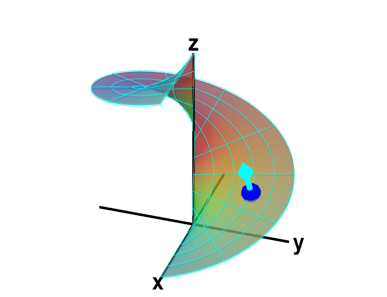
Let's illustrate this with the function \begin{align*} \dlsp(\spfv,\spsv) = (\spfv\cos \spsv, \spfv\sin \spsv, \spsv). \end{align*} that parametrizes a helicoid for $(\spfv,\spsv) \in \dlr = [0,1] \times [0, 2\pi]$. As shown in the following figure, we chose the upward point normal vector. (We could have used the downward point normal instead. If we did, our fluid flux calculation we have the opposite sign.)

Applet loading
Applet loading
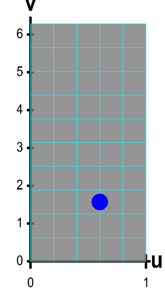
A parametrized helicoid with normal vector. The function $\dlsp(\spfv,\spsv) = (\spfv\cos \spsv, \spfv\sin \spsv, \spsv)$ parametrizes a helicoid when $(\spfv,\spsv) \in \dlr$, where $\dlr$ is the rectangle $[0,1] \times [0, 2\pi]$ shown in the first panel. The cyan vector at the blue point $\dlsp(\spfv,\spsv)$ is the upward pointing unit normal vector at that point. You can drag the blue point in $\dlr$ or on the helicoid to specify both $\spfv$ and $\spsv$.
Given some fluid flow $\dlvf$, if we integrate $\dlvf \cdot \vc{n}$, we will determine the total flux of fluid through the helicoid, counting flux in the direction of $\vc{n}$ as positive and flux in the opposite direction as negative.
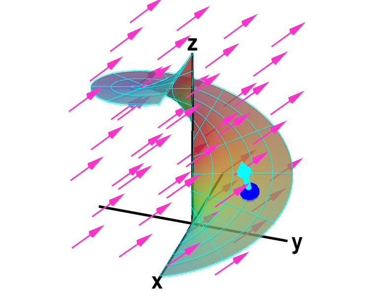
We represent the fluid flow vector field $\dlvf$ by magenta arrows in the following applet.

Applet loading
Applet loading
Fluid flow through oriented helicoid. The function $\dlsp(\spfv,\spsv) = (\spfv\cos \spsv, \spfv\sin \spsv, \spsv)$ parametrizes a helicoid when $(\spfv,\spsv) \in \dlr$, where $\dlr$ is the rectangle $[0,1] \times [0, 2\pi]$ shown in the first panel. The cyan vector at the blue point $\dlsp(\spfv,\spsv)$ is the upward pointing unit normal vector at that point. The magenta vector field represents fluid flow that passes through the surface. In this example, the vector field is the constant $\dlvf=(0,1,1)$. You can drag the blue point in $\dlr$ or on the helicoid to specify both $\spfv$ and $\spsv$.
It appears that the fluid is flowing generally in the same direction as $\vc{n}$ (for the most part $\dlvf$ and $\vc{n}$ are closer to pointing in the same direction than pointing in the opposite direction). However, notice, for example, that when $\spfv=0$ and $\spsv=2\pi$ (or when $\spfv=0$ and $\spsv=0$), the fluid is flowing in the opposite direction of $\vc{n}$ (at least the flow is closer to the opposite direction than the same direction). At these points, the fluid is crossing the surface in the opposite direction than it is at most points on the surface.
The below figure demonstrates this more clearly. Here, you can see the fluid vector $\dlvf$ (in magenta) at the same point as the normal vector (in cyan). The value of the flux $\dlvf \cdot \vc{n}$ across the surface at the blue point is shown in the lower right corner. Note that $\dlvf \cdot \vc{n}$ is usually positive, but is negative at a few points, such as those mentioned above. When $\dlvf \cdot \vc{n}=0$, what is the relationship between the fluid vector $\dlvf$ and the surface?
Applet loading

Applet loading
Fluid flow through a point of oriented helicoid. The function $\dlsp(\spfv,\spsv) = (\spfv\cos \spsv, \spfv\sin \spsv, \spsv)$ parametrizes a helicoid when $(\spfv,\spsv) \in \dlr$, where $\dlr$ is the rectangle $[0,1] \times [0, 2\pi]$ shown in the first panel. The cyan vector at the blue point $\dlsp(\spfv,\spsv)$ is the upward pointing unit normal vector at that point. The magenta vector at that point represents fluid flow that passes through the surface. In this case, the fluid flow is the constant $\dlvf=(0,1,1)$ at every point. Even though the fluid flow is constant, the flux through the surface changes, as it is the component of the flow normal to the surface. At the location of the blue point, the flux through the surface, $\dlvf \cdot \vc{n}$, is shown in the lower right corner. You can drag the blue point in $\dlr$ or on the helicoid to specify both $\spfv$ and $\spsv$.
The total flux of fluid flow through the surface $\dls$, denoted by $\dsint$, is the integral of the vector field $\dlvf$ over $\dls$. The integral of the vector field $\dlvf$ is defined as the integral of the scalar function $\dlvf \cdot \vc{n}$ over $\dls$ \begin{align*} \text{Flux} &= \dsint = \ssint{\dls}{\dlvf \cdot \vc{n}}. \end{align*} The formula for a surface integral of a scalar function over a surface $\dls$ parametrized by $\dlsp$ is \begin{align*} \ssint{\dls}{f} = \iint_\dlr f(\dlsp(\spfv,\spsv))\left\| \pdiff{\dlsp}{\spfv}(\spfv,\spsv) \times \pdiff{\dlsp}{\spsv}(\spfv,\spsv) \right\| d\spfv\,d\spsv. \end{align*}
Plugging in $f = \dlvf \cdot \vc{n}$, the total flux of the fluid is \begin{align*} \dsint= \iint_\dlr (\dlvf \cdot \vc{n}) \left\| \pdiff{\dlsp}{\spfv} \times \pdiff{\dlsp}{\spsv} \right\| d\spfv\,d\spsv. \end{align*}
Lastly, the formula for a unit normal vector of the surface is \begin{align*} \vc{n} = \frac{\displaystyle \pdiff{\dlsp}{\spfv} \times \pdiff{\dlsp}{\spsv}}{\displaystyle \left\| \pdiff{\dlsp}{\spfv} \times \pdiff{\dlsp}{\spsv} \right\|}. \end{align*} If we plug in this expression for $\vc{n}$, the $\left\| \pdiff{\dlsp}{\spfv} \times \pdiff{\dlsp}{\spsv} \right\|$ factors cancel, and we obtain the final expression for the surface integral: \begin{align*} \dsint= \iint_\dlr \dlvf(\dlsp(\spfv,\spsv)) \cdot \left( \pdiff{\dlsp}{\spfv}(\spfv,\spsv) \times \pdiff{\dlsp}{\spsv}(\spfv,\spsv) \right) d\spfv\,d\spsv. \label{eq:surfvec} \end{align*}
Note how the equation for a surface integral is similar to the equation for the line integral of a vector field \begin{align*} \dlint = \int_a^b \dlvf(\dllp(t)) \cdot \dllp'(t) dt. \end{align*} For line integrals, we integrate the component of the vector field in the tangent direction given by $\dllp'(t)$. For surface integrals, we integrate the component of the vector field in the normal direction given by $\pdiff{\dlsp}{\spfv}(\spfv,\spsv) \times \pdiff{\dlsp}{\spsv}(\spfv,\spsv)$.
You can read some examples of calculating surface integrals of vector fields.
Thread navigation
Multivariable calculus
- Previous: Introduction to a surface integral of a scalar-valued function
- Next: Scalar surface integral examples
Math 2374
- Previous: Scalar surface integral examples
- Next: Vector surface integral examples
Notation systems
Similar pages
- Introduction to a surface integral of a scalar-valued function
- Scalar surface integral examples
- Vector surface integral examples
- The integrals of multivariable calculus
- Introduction to double integrals
- Double integrals as iterated integrals
- Double integral examples
- Double integrals as volume
- Examples of changing the order of integration in double integrals
- Double integrals as area
- More similar pages