Introduction to a surface integral of a scalar-valued function
There are many parallels between parametrized surfaces and parametrized curves. Both are parametrized by vector-valued functions, with the difference being the dimension of their inputs (one-dimensional $t$ for parametrized curves and two-dimensional $(\spfv,\spsv)$ for parametrized surfaces). Both have two possible orientations (oriented by choice of tangent vector for curves and by choice of normal vector for surfaces). Both have integrals giving their measure (arc length or area) in terms of derivatives of the parametrization that describe how the domain is stretched and shrunk as it is mapped onto the image.
In the same way, surface integrals are similar to line integrals. Just as there are two types of integrals over curves (line integrals of scalar functions and of vector fields) there are two types of surface integrals: surface integrals of scalar functions (discussed on this page) and surface integrals of vector fields. The surface integral of a scalar function is a simple generalization of a double integral. Like the line integral of vector fields, the surface integrals of vector fields will play a big role in the fundamental theorems of vector calculus.
Let $\dls$ be a surface parametrized by $\dlsp(\spfv,\spsv)$ for $(\spfv,\spsv)$ in some region $\dlr$. Imagine you wanted to calculate the mass of the surface given its density at each point $\vc{x}$ described by the scalar-valued function $f(\vc{x})$. The mass will be the integral of the density over the surface (just like the mass of a wire was the integral of a density over the curve).
If the surface happened to be lying in the $xy$-plane rather than floating in three-dimensional space, the situation would be identical to that of changing variables in double integrals (other than the region we call $\dlr$ here is called $\dlr^*$ in that context changing variables). We need only slight modifications for the case of a surface floating in three dimensional space.
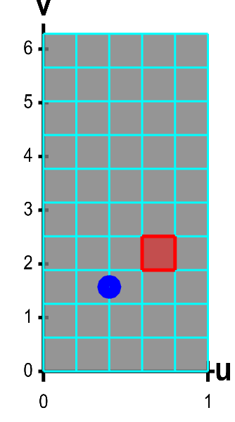
To calculate the mass, we integrate $f(\dlsp(\spfv,\spsv))$ as $(\spfv,\spsv)$ range over the domain $\dlr$. In order to multiply the density $f$ by area on the surface not by area in $\dlr$, we must account for any stretching or shrinking by $\dlsp$ as it maps $\dlr$ onto the surface, as illustrated in the below applet.
Applet loading
Applet loading
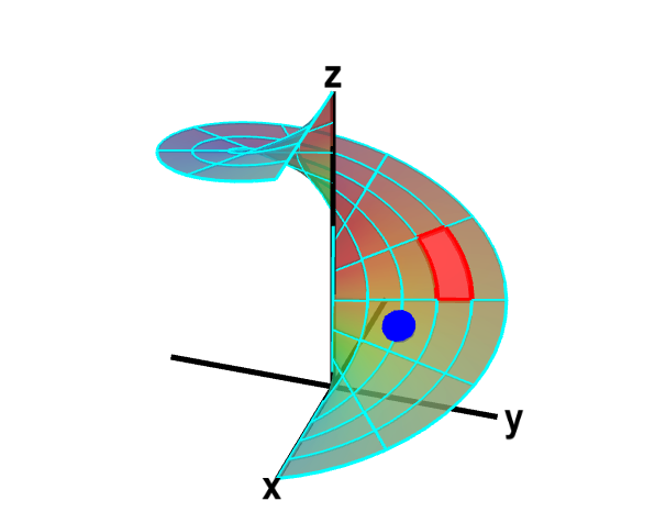
A parametrized helicoid with surface area elements. The function $\dlsp(\spfv,\spsv) = (\spfv\cos \spsv, \spfv\sin \spsv, \spsv)$ parametrizes a helicoid when $(\spfv,\spsv) \in \dlr$, where $\dlr$ is the rectangle $[0,1] \times [0, 2\pi]$. The region $\dlr$, shown as the rectangle on the left, is divided into small rectangles, which are mapped onto “curvy rectangles” on the surface at the right. To visualize the mapping, you can click on a rectangle in either panel to highlight it in red; the corresponding rectangle in the opposite panel is also hightlighted in red. The area of the red region on the helicoid depends on how $\dlsp$ stretches or shrinks the small red rectangle of $\dlr$ as it maps it on the surface. You can also drag the blue point in either $\dlr$ or the helicoid surface, and the blue point in the opposite panel moves so that the location of the right point is $\dlsp(\spfv,\spsv)$ when the location of the left point is $(\spfv,\spsv)$.
We already calculated the stretching or shrinking by $\dlsp$ when we calculated surface area. The area of the region on the surface that is the image of a small $\Delta\spfv \times \Delta\spsv$ rectangle in $\dlr$ is \begin{align*} \Delta A = \left\| \pdiff{\dlsp}{\spfv}(\spfv,\spsv) \times \pdiff{\dlsp}{\spsv}(\spfv,\spsv) \right\| \Delta \spsv \Delta \spsv. \end{align*} If we multiply this by the density $f(\dlsp(\spfv,\spsv))$, we will obtain the mass of that small section. We could approximate the mass of the whole surface by a Riemann sum of such terms. Then, by letting $\Delta\spfv$ and $\Delta\spsv$ go to zero, we would discover that the mass of the whole surface is the integral \begin{align*} \ssint{\dls}{f} = \iint_\dlr f(\dlsp(\spfv,\spsv))\left\| \pdiff{\dlsp}{\spfv}(\spfv,\spsv) \times \pdiff{\dlsp}{\spsv}(\spfv,\spsv) \right\| d\spfv\,d\spsv. \end{align*} This integral is a two-dimensional analog of the line integral of a scalar-valued function except that $\|\dlsp'(t)\|$ is replaced by \begin{align*} \left\| \pdiff{\dlsp}{\spfv}(\spfv,\spsv) \times \pdiff{\dlsp}{\spsv}(\spfv,\spsv) \right\|. \end{align*}
You can read some examples of calculating surface integrals of scalar functions.
Thread navigation
Multivariable calculus
Math 2374
- Previous: A Möbius strip is not orientable
- Next: Scalar surface integral examples
Notation systems
Similar pages
- Introduction to a surface integral of a vector field
- Scalar surface integral examples
- Vector surface integral examples
- The integrals of multivariable calculus
- Introduction to double integrals
- Double integrals as iterated integrals
- Double integral examples
- Double integrals as volume
- Examples of changing the order of integration in double integrals
- Double integrals as area
- More similar pages