The idea behind Green's theorem
When $\dlc$ is an oriented simple closed curve, the integral \begin{align*} \dlint \end{align*} represents the circulation of $\dlvf$ around $\dlc$. If $\dlvf$ were the velocity field of water flow, for example, this integral would indicate how much the water tends to circulate around the path in the direction of its orientation.
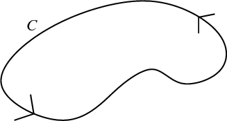
One way to compute this circulation is, of course, to compute the line integral directly. But, if our line integral happens to be in two dimensions (i.e., $\dlvf$ is a two-dimensional vector field and $\dlc$ is a closed path that lives in the plane), then Green's theorem applies and we can use Green's theorem as an alternative way to calculate the line integral.
Green's theorem transforms the line integral around $\dlc$ into a double integral over the region inside $\dlc$. However, it's not obvious what function we should integrate over the region inside $\dlc$ so that we still get the same answer as the line integral. The notion of circulation can aid us in determining what this function should be.
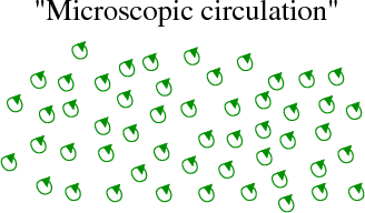
Think of the integral $\dlint$ as the “macroscopic” circulation of the vector field $\dlvf$ around the path $\dlc$. Now, imagine you came up with a “microscopic” version of circulation around a curve. This microscopic circulation at a point $(x,y)$ has to tell you how much $\dlvf$ would circulate around a tiny closed curve centered around $(x,y)$. We could picture the microscopic circulation as a bunch of small closed curves (shown below in green), where each curve respresents the tendency for the vector field to circulate at that location (imagine that the small curves were really, really small, much smaller than pictured).
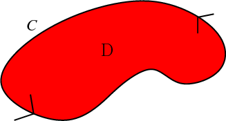
Green's theorem is simply a relationship between the macroscopic circulation around the curve $\dlc$ and the sum of all the microscopic circulation that is inside $\dlc$. If $\dlc$ is a simple closed curve in the plane (remember, we are talking about two dimensions), then it surrounds some region $\dlr$ (shown in red) in the plane. $\dlr$ is the “interior” of the curve $\dlc$.
Green's theorem says that if you add up all the microscopic circulation inside $\dlc$ (i.e., the microscopic circulation in $\dlr$), then that total is exactly the same as the macroscopic circulation around $\dlc$.
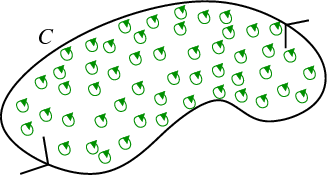
“Adding up” the microscopic circulation in $\dlr$ means taking the double integral of the microscopic circulation over $\dlr$. Therefore, we can write Green's theorem as \begin{align*} \dlint = \iint_\dlr \text{“microscopic circulation of $\dlvf$” } dA. \end{align*}
What is this microscopic circulation? The microscopic circulation of Green's theorem is the same as the microscopic circulation of the curl of a three-dimensional vector field. The only difference is that Green's theorem applies only with two-dimensional vector fields, e.g., for vector fields in the $xy$-plane. The microscropic circulation we want is circulation in the $xy$-plane.
Microscopic circulation in the $xy$ plane turns out to be the $z$-component of the curl. You can see this as follows. The direction of the curl and the definition of its components is determined by the right-hand rule. (Imagine curling the fingers of your right hand around the circles indicating the circulation. One represents such circulation by a vector pointing in the direction of your thumb.) In three-dimensions, point the thumb of your right hand in the positive $z$ direction. Then, the fingers of your right hand curl in the counterclockwise direction parallel to the $xy$-plane. So, the right-hand rule says that circulation in the $xy$-plane should correspond to the $z$-component of the curl.
We conclude that, for Green's theorem, \begin{align*} \text{“microscopic circulation”} = (\curl \dlvf) \cdot \vc{k}, \end{align*} (where $\vc{k}$ is the unit vector in the $z$-direction) and we can write Green's theorem as \begin{align*} \dlint = \iint_\dlr (\curl \dlvf) \cdot \vc{k} \, dA. \end{align*}
The component of the curl in the $z$-direction is given by the formula \begin{align*} (\curl \dlvf) \cdot \vc{k} = \pdiff{\dlvfc_2}{x} - \pdiff{\dlvfc_1}{y}. \end{align*} This $z$-component of the curl is often termed the scalar curl of a two-dimensional vector field. You can get intuition behind this formula or see how to derive this formula from the definition of the curl. Using this formula, we can write Green's theorem as \begin{align*} \dlint = \iint_\dlr \left( \pdiff{\dlvfc_2}{x} - \pdiff{\dlvfc_1}{y}\right)dA. \end{align*}
To make sure that Green's theorem gives the right answer, we need to be careful how we orient the curve $\dlc$. The right hand rule says that $(\curl \dlvf) \cdot \vc{k}$ corresponds to the amount of circulation in the counterclockwise direction. Hence, Green's theorem, as we have written it, is valid only for curves oriented counterclockwise (as pictured above). In this case, we say that $\dlc$ is a positively oriented boundary of the region $\dlr$. One way to remember what positively oriented means is the following: if you were to walk along $\dlc$ in the positive orientation, the region $\dlr$ will be to your left. If you mess up the orientation, you'll be off by a minus sign.
Green's theorem and other fundamental theorems
Green's theorem is one of the four fundamental theorems of vector calculus all of which are closely linked. Once you learn about surface integrals, you can see how Stokes' theorem is based on the same principle of linking microscopic and macroscopic circulation.
What if a vector field had no microscopic circulation? Looking at Green's theorem, we immediately see if this microscopic circulation $\pdiff{\dlvfc_2}{x} - \pdiff{\dlvfc_1}{y}$ were zero in some region $\dlr$, then the line integral \begin{align*} \int_\dlc \dlvf \cdot d\vc{s}=0 \end{align*} for any closed curve $\dlc$ in $\dlr$ (for example, the closed curve $\dlc$ that is the boundary of $\dlr$). This is a property of conservative or path-independent vector fields, which forms the basis for the gradient theorem for line integrals.
Are you ready to use Green's theorem? Make sure you understand when you are allowed to use Green's theorem, check out some other ways of writing Green's theorem, then investigate some examples. To become a master at Green's theorem, you should understand how it applies to more general regions with holes.
Thread navigation
Multivariable calculus
- Previous: Finding a potential function for three-dimensional conservative vector fields
- Next: When Green's theorem applies
Math 2374
Notation systems
Similar pages
- Calculating the formula for circulation per unit area
- Line integrals as circulation
- Using Green's theorem to find area
- The definition of curl from line integrals
- A path-dependent vector field with zero curl
- The idea behind Stokes' theorem
- The idea of the curl of a vector field
- Subtleties about curl
- The components of the curl
- Introduction to a line integral of a vector field
- More similar pages