Vector fields as fluid flow

As described in the vector field overview, a two-dimensional vector field is a vector-valued function $\dlvf:\R^2 \to \R^2$ (confused?) that one can visualize with a field of arrows. For example, the below graph is a visualization of the vector field $\dlvf(x,y)=(y,-x)$.

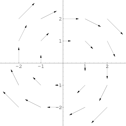
One can think of such a vector field as representing fluid flow in two dimensions, so that $\dlvf(x,y)$ gives the velocity of a fluid at the point $(x,y)$. In this case, we may call $\dlvf(x,y)$ the velocity field of the fluid. With this interpretation, the above example illustrates the clockwise circulation of fluid around the origin.

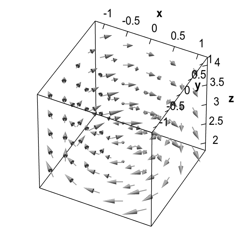
The same interpretation is possible for a three-dimensional fluid flow with velocity represented by a vector field $\dlvf:\R^3 \to \R^3$. In this case, $\dlvf(x,y,z)$ is the velocity of the fluid at the point $(x,y,z)$, and we can visualize it as the vector $\dlvf(x,y,z)$ positioned a the point $(x,y,z)$. For example, $\dlvf(x,y,z)=(y/z,-x/z,0)$ can be viewed as fluid circulating around the $z$-axis.

The Java applet did not load, and the above is only a static image representing one view of the applet. The applet was created with LiveGraphics3D. The applet is not loading because it looks like you do not have Java installed. You can click here to get Java.

A three-dimensional rotating vector field. You can rotate the graph with the mouse to give perspective.

The interpretation of vector fields as fluid flow can be useful in understanding basic properties of vector fields, such as divergence and curl, as well as important results in vector analysis, such as Green's theorem and Stokes' theorem.