How linear transformations map parallelograms and parallelepipeds
The notion of linearity plays an important role in calculus because any differentiable function is locally linear, i.e., looks linear if you zoom in enough. In fact, the definition of differentiability is based on the ability to approximate a function $\vc{f}(\vc{x})$ by a linear transformation $\vc{T}(\vc{x})$.
Here we discuss a simple geometric property of linear transformations. A two-dimensonal linear transformation maps parallelograms onto parallelograms and a three-dimensional linear transformation maps parallelepipeds onto parallelepipeds. This property, combined with the fact that differentiable functions become approximately linear when one zooms in on a small region, forms the basis for calculating the area or volume transformation when changing variables in double or triple integrals as well as calculating area for parametrized surfaces.
Mapping parallelograms in two dimensions
A two-dimensional linear transformation $\vc{T}: \R^2 \to \R^2$ (confused?) is a type of mapping from a two-dimensional plane onto another two-dimensional plane. It can be written as $$\vc{T}(x,y) = (ax+by,cx+dy) = \left[\begin{array}{cc}a &b\\ c &d\end{array}\right]\left[\begin{array}{c}x\\y\end{array}\right],$$ where $a$, $b$, $c$, and $d$ are numbers defining the linear transformation, or more succinctly as $$\vc{T}(\vc{x}) = A\vc{x},$$ where $\vc{x}=(x,y)$ and $A$ is the $2 \times 2$ matrix $$A = \left[\begin{array}{cc}a &b\\ c &d\end{array}\right].$$
We can view $\vc{T}$ as mapping regions from the $xy$-plane onto an $x'y'$-plane: $(x',y')=\vc{T}(x,y)$. You can experiment with this mapping by a linear transformation in the following applet.
Linear transformation in two dimensions. The linear transformation $\vc{T}=A\vc{x}$, with $A$ specified in the upper left hand corner of the applet, is illustrated by its mapping of a quadrilateral. The original quadrilateral is shown in the $xy$-plane of the left panel and the mapped quadrilateral is shown in the $x'y'$-plane of the right panel. You can change the linear transformation by typing in different numbers and change either quadrilateral by moving the points at its corners. The determinant of $A$ (shown in upper left hand corner) determines how much $\vc{T}$ stretches or compresses area and whether or not it reverses the orientation of the region. The orientation of each quadrilateral can be determined by examining the order of the colors while moving in a counterclockwise direction around its perimeter. Use the + and - buttons of each panel to zoom in and out. (When $\det A =0$, you cannot drag points in the right panel.)
The first thing to notice the linear transformation maps quadrilaterals onto quadrilaterals. Unlike a nonlinear transformation, which can bend straight lines into curves, a linear transformation maps straight lines onto straight lines. This fact is easily seen by thinking of a parametrization of a line, such as $$\vc{x} = t \vc{v} + \vc{a}.$$ Given a linear transformation $\vc{x}' = \vc{T}\vc{x} = A\vc{x}$, we can multiply the line parametrization equation by the matrix $A$ associated with the linear transformation, yielding $$A\vc{x} = t A\vc{v} + A\vc{a}.$$ If we let $\vc{v}'=A\vc{v}$ and $\vc{a}' = A\vc{a}$ be the images of the vectors $\vc{v}$ and $\vc{a}$ under the linear transformation, then the parametrization in terms of the transformed variables $\vc{x}'$ is simply $$\vc{x}' = t \vc{v}' + \vc{a}'$$ which is clearly also a parametrization of a line.
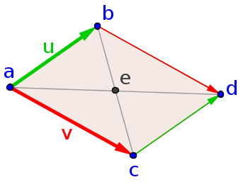
We want to show a stronger condition, though, namely that the linear transformation $\vc{T}$ always maps parallelograms onto parallelograms. Starting with a parallelogram spanned by the vectors $\vc{u}$ and $\vc{v}$ with one vertex at the point $\vc{a}$, illustrated below, we can calculate that the image of this parallelogram under $\vc{T}$ must also be a parallelogram. Since we already know that the edges will be straight lines, we simply need to show that the vertices of the parallelogram are mapped to locations corresponding to vertices of another parallelogram.
We label the vertices neighboring $\vc{a}$ as $\vc{b}=\vc{a}+\vc{u}$ and $\vc{c}=\vc{a}+\vc{v}$. What makes the quadrilateral a parallelogram is that the fourth vertex $\vc{d}$ is constrained to be equal to the first vertex $\vc{a}$ plus the vectors from $\vc{a}$ to both $\vc{b}$ and $\vc{c}$, i.e., $\vc{d} = \vc{a}+\vc{u}+\vc{v}$. In terms of just the vertices, we can write the condition for the parallelogram as $\vc{d} = \vc{b}+\vc{c}-\vc{a}$. Or, if we don't want to make any vertex special, we could write the condition as $\vc{d}+\vc{a} = \vc{b}+\vc{c}$. The sums of the opposite vertices must be the same, or equivalently, the midpoints of opposite vertices must be the same point, labeled as $\vc{e}$ in the figure. (We can add points because here, as always, we equate a point with the vector whose tail is at the origin and head is at the point.)
In order to show that the image of the parallelogram under $\vc{T}$ is still a parallelogram, we simply need to show that the same relationship among the vertices still holds. Label the vertices of the image quadrilateral as $\vc{a}'=\vc{T}(\vc{a})$, $\vc{b}'=\vc{T}(\vc{b})$, $\vc{c}'=\vc{T}(\vc{c})$, and $\vc{d}'=\vc{T}(\vc{d})$. Given the condition $\vc{d}+\vc{a} = \vc{b}+\vc{c}$, which means the original quadrilateral is a parallelogram, we can multiply the condition by the matrix $A$ associated with $\vc{T}$ and obtain that $A\vc{d}+A\vc{a} = A\vc{b}+A\vc{c}$. Rewriting this expression in terms of the new vertices, this equation is exactly $\vc{d}'+\vc{a}' = \vc{b}'+\vc{c}'$. Indeed, the image of a parallelogram under a linear transformation is another parallelogram.
Mapping parallelepipeds in three dimensions
A three-dimensional linear transformation is a function $\vc{T}: \R^3 \to \R^3$ of the form $$\vc{T}(x,y,z) = (a_{11}x+a_{12}y + a_{13}z, a_{21}x+a_{22}y+a_{23}z,a_{31}x+a_{32}y+a_{33}z) = A\vc{x}.$$ where $$A=\left[\begin{array}{ccc}a_{11}&a_{12}&a_{13}\\a_{21}&a_{22}&a_{23}\\a_{31}&a_{32}&a_{33}\end{array}\right]$$ and $\vc{x}=(x,y,z)$. The components $a_{ij}$ of $A$ define the linear transformation.
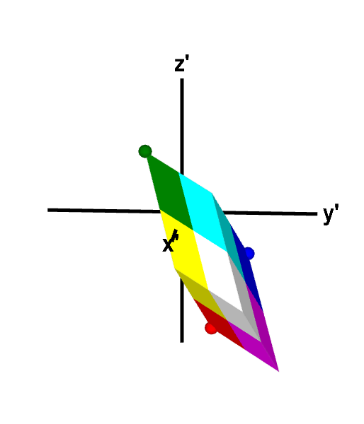
An example of such a three-dimensional linear transformation is shown in the following applet. The original region is constrained to be a parallelepiped, and you can observe that is always mapped to another parallelepiped.

Applet loading
Applet loading
A three-dimensional linear transformation that preserves orientation. The linear transformation $\vc{T}(\vc{x}) = A\vc{x}$, where $$A=\left[\begin{array}{rrr}2&1&1\\1&2&-1\\-3&-1&2\end{array}\right]$$ maps the unit cube to a parallelepiped of volume 12. The expansion of volume by $\vc{T}$ is reflected by that fact that $\det A = 12$. Since $\det A$ is positive, $\vc{T}$ preserves orientation, as revealed by the face coloring of the cube and parallelogram. The order of the colors on corresponding faces, when moving in a counterclockwise direction, is the same for both the cube and the parallelepiped. For example, both objects have a face with the counterclockwise color order blue, magenta, white, cyan. You can further explore the mapping by changing either shape to other parallelepipeds by dragging the points on four of its vertices.
We don't need to do any additional work to demonstrate that linear transformations in three-dimensions map parallelepipeds onto parallelepipeds. Since the above calculations were not specific to two dimensions, they demonstrate that three-dimensional linear transformations map parallelograms onto parallelograms. Therefore, $\vc{T}$ maps the six parallelogram faces of a parallelepiped onto six other parallelograms. This result means that $\vc{T}$ maps the parallelepiped onto a three-dimensional geometric solid with six faces that are parallelograms, which is the definition of a parallelepiped. We can conclude that linear transformations map parallelepipeds onto parallelepipeds.
Thread navigation
Vector algebra
- Previous: Geometric properties of the determinant
- Next: Parametrization of a line
Math 2374
- Previous: Geometric properties of the determinant
- Next: Level sets*
Similar pages
- Determinants and linear transformations
- Matrices and linear transformations
- Linear transformations
- Geometric properties of the determinant
- Polar coordinates mapping
- Parametrization of a line
- Parametrization of a line examples
- Matrices and determinants for multivariable calculus
- The definition of differentiability in higher dimensions
- Subtleties of differentiability in higher dimensions
- More similar pages